RetractorDB
RetractorDB is an Edge Signal Processing Engine (ESPE) designed to continuously process regular time series close to the data source. Its declarative RQL language describes transformations, aggregations, and rules; their results can be published live or materialized as artifacts that remain available for later inspection and correction. The system complements central time-series databases and stream-processing systems by reducing the volume of data sent to them, but it does not replace those systems.
The name combines two ideas. Retractor denotes a tool that extracts, separates, joins, and processes data contained in time series, while DB points to mechanisms familiar from databases: a declarative query language, schema descriptions, access methods, and persistent result storage. The origin of the name is explained in Why Was This Name Chosen for the System?.
This documentation leads from the mathematical foundations and the construction of RQL, through the system architecture, query compilation and execution, to application examples and reference appendices. First-time readers should follow the chapter order in the table of contents because later sections build on concepts introduced earlier. Readers looking for a specific solution can go directly to the relevant chapter, then use the examples and appendices as practical and reference material.
RetractorDB among neighboring fields
This chapter is a map, not a catalog. Instead of listing everything ever written about streams and signals, I show eight strands of research literature at whose intersection RetractorDB sits, and for each of them I answer three questions: what has this strand already solved, how does RetractorDB differ from it, and what does this strand not touch. Comparing them reveals the gap this project fills.
📥 Download the documentation
This documentation is compiled entirely from Markdown files. Three targets are copied. The first is the HTML page you see now, the second is the PDF file, and the third is the EPUB document for the reader. Each time the content of the GitHub repository where the Markdown files are stored changes, a process is triggered to create these three targets.
✅ Note
This system is an: Edge Signal Processing Engine. RetractorDB supports - rather than replaces - time-series databases (TSDB) and data stream management systems (DSMS): it works close to the signal source, pre-processes and filters high-frequency measurements using a declarative query language, keeps a partial, correctable record of past events and scheduled future ones in inspectable artifacts, and passes exact, deterministic results up the architecture - so that only reduced, already-processed streams reach the central architecture.
ℹ️ Info
Why did I place this chapter so early? Because an honest answer to the question “is this needed?” first requires showing what already exists. Most ideas in computer science have already been thought of once - reinventing the wheel wastes someone else’s effort. This chapter is my attempt to prove that this particular wheel has not, in fact, been invented yet.
Eight neighboring fields
The problem RetractorDB solves does not belong entirely to any single discipline. It lies at the intersection of eight strands:
-
1. Number theory
Beatty sequences, Fraenkel’s theorem, covering systems. This provides the formal foundation.
-
2. Task scheduling via Beatty sequences
The same mathematics, a different application. The closest application-level neighbor.
-
3. Synchronous and cyclo-static dataflow (SDF/CSDF)
Multirate actor graphs, static schedules, and buffer bounds.
-
4. Synchronous languages and clock calculi
Declarative relations between periodic streams and compile-time delay inference.
-
5. Digital signal processing (DSP)
Nonuniform sampling and filter banks with rational coefficients. This is the DSP counterpart of the interleaving operation.
-
6. Data stream management systems (DSMS)
Stream algebras and continuous-query semantics. This is the database reference point.
-
7. Multi-query sharing and shared state
Reuse of computation, indexes, and materializations across plans.
-
8. Time-series systems (TSMS) and in-database DSP
The narrowest niche, closest to the system’s actual goal.
I discuss them in turn, from the foundation toward the application.
Number theory: Beatty sequences and covering systems (1)
RetractorDB’s entire algebra rests on the Beatty sequence and its generalization by Fraenkel to rational numbers. I cite these results in Formal Foundations and Proofs. Here I’m interested in the broader backdrop: how this mathematics functions in the contemporary literature, and whether anyone has already applied it where I have.
Beatty sequences have a rich combinatorial literature and documented applications in aperiodic tilings (quasicrystals), periodic scheduling, computer vision (digital lines), and formal language theory [11]. The strand is alive: Schaeffer, Shallit, and Zorcic (2024) showed that a non-homogeneous Beatty sequence is synchronizable by a finite automaton, which leads to decidability of the first-order theory of these sequences [12]. For me, however, the most relevant work is that of Berger, Felzenbaum, and Fraenkel (1986) on disjoint covering systems based on rational Beatty sequences [13] - exactly the variant my de-interleaving is based on, and one I did not cite in the original paper.
What this strand does not touch: number theory studies these sequences as mathematical objects. It does not connect them to a database, to a stream-processing model, or to signal processing. It supplies bricks, not a building.
Task scheduling via Beatty sequences (2)
This is the strand I must discuss most honestly, because it uses the same proof machinery as my theorems - just for a different purpose. In the periodic-scheduling problem (so-called pinwheel scheduling), tasks with different repeat periods are distributed so that tasks with one repeat time land in time slots belonging to the first complementary Beatty sequence, and those with the other, into the second [14]. Recent work (2025) proves results on the Rayleigh/Beatty partition using identities on floor and ceiling functions of the type ⌈(m+l)a⌉ − ⌈ma⌉ [15] - almost identical, point for point, to the apparatus in my proof that de-interleaving satisfies Fraenkel’s postulates.
The conclusion, for me, is twofold. On one hand - this is independent confirmation that the approach is correct and natural; if someone else arrives, by the same road, at a working scheduling scheme, the foundation is solid. On the other - it narrows what I can call novel. “Beatty sequences for scheduling” already exists and is being actively published. Interestingly, my system uses this mathematics internally, precisely for task scheduling (see Query Execution) - but that’s not where the original contribution lies.
What this strand does not touch: scheduling treats sequences as a tool for allocating time slots to processors. It doesn’t build a data algebra on top of them, doesn’t use them to express operations on signals, and doesn’t create a query language.
Synchronous and cyclo-static dataflow (SDF/CSDF) (3)
In SDF, actors consume and produce statically known token counts, which makes it possible to derive a graph schedule before execution [26]. CSDF extends this model with cyclically changing production and consumption rates and supports static schedules and buffer bounds [27]. This is a mature model of declarative multirate dataflow, so neither rate analysis nor static scheduling is unique to RetractorDB.
SDF/CSDF can describe related multirate behavior, which justifies the “partial” assessment for lossless sample partition. A Beatty partition is not, however, a distinct semantic operator in those models. RetractorDB places that operator in a query language and connects it to persistent results.
What this strand does not touch: SDF/CSDF does not define this particular lossless partition of sample positions as the semantics of a query system or provide an artifact inspection and replay model around it.
Synchronous languages and clock calculi (4)
Synchronous languages describe periodic streams through clocks and can check their compatibility and derive required buffers and delays during compilation. In n-synchronous models, clock relations may have rational rate ratios, and the compiler takes over part of the synchronization burden [28]. This is one of the closest reference points for RetractorDB’s declarative boundary.
The object being described is different, however: a clock usually marks whether a value is present at a logical tick, whereas RetractorDB assigns a rational interval to a regular stream and uses it to form one ordered stream from two inputs.
What this strand does not touch: clock calculi primarily support the compilation of reactive programs. They do not carry this semantics into a query engine with public descriptors and persistent, replayable artifacts.
Digital signal processing: nonuniform sampling and filter banks (5)
Interleaving and de-interleaving meet DSP in the problem of working with streams at different sampling rates, but they are not simply another signal-reconstruction method. The closest bridge is the work of Samadi, Ahmad, and Swamy (2004), which formulates the perfect-reconstruction condition for nonuniform filter banks from the system’s response to delayed unit-step signals [16]. The broader strand includes periodic nonuniform sampling of band-limited signals [17] and filter banks with rational decimation factors (Kovačević and Vetterli) [18].
Number-theoretic constructions even show up there: Ramanujan filter banks extract periodic components of a signal [19]. But I have not found Beatty sequences or Fraenkel’s theorem specifically in this literature - and that’s part of the gap.
What this strand does not touch: the cited DSP methods reconstruct or transform signal values. They do not define this particular Beatty-based interleaving of sample positions or embed it in an artifact-producing query engine.
Data stream management systems (DSMS) (6)
On the database side, the canon is CQL from Stanford’s STREAM project (Arasu, Babu, Widom). In this model, a stream is a potentially infinite multiset of elements ⟨s, τ⟩, where s is a tuple and τ a timestamp [20]; query semantics is built on windows and stream↔relation mappings. A second close neighbor is the temporal algebra of Krämer and Seeger (the PIPES system), providing deterministic results for continuous queries and a rich set of transformation rules underlying optimization [21].
This is the proper reference point for my algebra and my expression rewrite rules. The difference, however, is fundamental and concerns the data model itself. CQL and PIPES build their semantics on the (s, τ) model - every tuple carries its own timestamp, and operators act through windows. I adopt a differential model (sₙ, Δ), with a rational, fixed value of Δ per stream, and I derive the operators that align streams with different Δ from number theory. This is not a cosmetic difference in syntax - it’s a different data model, leading to a different class of operators (interleaving, de-interleaving) and a different optimization method.
In deployment terms, the relationship is complementary rather than competitive: RetractorDB acts as an edge-level pre-processing and buffering stage, whose exact, deterministic results can feed a windowed DSMS.
What this strand does not touch: DSMS encompass both deterministic semantics and mechanisms for scaling, windows, out-of-order handling, and state management. The cited systems do not, however, define this particular lossless partition of regular sample positions using Beatty sequences or use number theory as the semantics of resampling.
Multi-query sharing and shared state (7)
Multi-query optimization has long reused common parts of query plans. More recent streaming systems also share maintained indexes and state across concurrent dataflows [29], while semantic normalization makes it possible to merge queries whose syntax or plan structure differs [30]. Automatic sharing is therefore not, by itself, a new contribution of RetractorDB.
In RetractorDB, this problem concerns materialized intermediate streams. The compiler may share them only after plan normalization and a compatibility check grounded in regular-series semantics. This is close to existing shared-state mechanisms, although the compatibility criterion here follows from the stream-rate model.
What this strand does not touch: the cited methods do not use rate alignment and a Beatty partition to normalize a plan before deciding whether to share. The detailed boundary of this comparison is beyond the scope of the system documentation.
Time-series systems (TSMS) and in-database DSP (8)
This is the narrowest niche - and the closest to RetractorDB’s actual goal. The canonical survey is Jensen, Pedersen, and Thomsen’s “Time Series Management Systems: A Survey” (IEEE TKDE, 2017) [22]. The Plato system described there is the closest real “DSP inside a database”: it combines an RDBMS with signal-processing methods, eliminating the need to export data to external tools like R or SPSS [22]. The other approaches to “signals in a database” boil down to approximation and compression - wavelet, dictionary, and shape-based representations.
These approaches focus on approximation, compression, or after-the-fact analytics. They do not make Beatty-based multiplexing of sample positions a first-class operator within a query algebra. RetractorDB does not compete with them on ingestion scale or retention: it runs ahead of a central system and supplies deterministic results and correctable artifacts.
What this strand does not touch: TSMS optimize ingestion scale, compression, and retention. DSP is a second-class citizen in them - an analytical add-on, not the core of the semantics.
The blank spot: where the contribution lies
The table below is a qualitative capability map, not evidence of priority or a claim that the review is complete. The final column concerns evaluation through inspectable artifacts or replay, not persistence alone. “Partial” denotes a related capability, not semantic equivalence.
| Field | Beatty/Fraenkel | Lossless sample partition | Declarative dataflow | Artifact / replay evaluation |
|---|---|---|---|---|
| Number theory | ✔ | – | – | – |
| Scheduling (pinwheel) | ✔ | – | – | partial |
| SDF / CSDF | – | partial | ✔ | – |
| Synchronous languages / clock calculi | – | – | ✔ | – |
| Multirate DSP | – | partial | partial | – |
| DSMS (CQL, PIPES) | – | – | ✔ | partial |
| Multi-query sharing / shared state | – | – | ✔ | partial |
| TSMS / in-database DSP | – | partial | partial | partial |
| RetractorDB | ✔ | ✔ | ✔ | ✔ |
The strongest neighbors in the execution-model dimension are SDF/CSDF and synchronous languages and clock calculi: they already provide multirate declarative dataflow, deterministic semantics, static schedules, or buffer inference. The multi-query strand is equally close along an axis not represented by the columns: it can share maintained state automatically and formulate preservation conditions for individual queries. Its “partial” entry understates that proximity because the table does not describe how the identity of a shared object is established.
RetractorDB’s integration scope is narrower: the system combines a Beatty-defined, exactly invertible partition of sample positions with a query compiler, a sequential slot runtime, and persistent artifacts that can be inspected and replayed. This describes the system’s architecture and semantics; it does not claim that the individual ingredients are new. RetractorDB does not claim hard real-time guarantees.
⚠️ Warning
Hence a real risk, which I point out directly: the scheduling community has been publishing this same Beatty/Fraenkel machinery in 2023–2025. The problem itself - together with the need for a declarative stream algebra and a continuous query language - was already formulated back in 2003–2005, in the context of computer-assisted fetal monitoring [25]; I laid the “covering systems ↔ stream alignment and DSP” bridge in a 2006 publication [3], but in a venue with low discoverability. If this result doesn’t reach well-cited circulation, the same bridge may be independently built and credited to someone else.
Methodological caveat
This is a targeted review, not a systematic one - based on searching across eight strands, not a full citation analysis. A “forward citation” review of Samadi’s paper [16] confirms the point: according to Semantic Scholar (as of July 2026), its only recorded citations are a paper on Gabor window design, two systems-theoretic papers on multirate systems, and the 2006 bridge paper itself [3] - none of them uses Beatty sequences or Fraenkel’s theorem. The closest use of this machinery outside number theory that I’m aware of is the construction of exponential Riesz bases from Beatty–Fraenkel sequences (Pfander, Revay, and Walnut) [24] - but that belongs to pure harmonic analysis and doesn’t touch filter banks or sample-rate conversion. What remains for full closure is a systematic review of the scheduling strand [14] and of the filter-bank literature as a whole; the query-sharing discussion cites representative mechanisms rather than attempting a complete catalog. If a use of Fraenkel’s theorem in multirate DSP exists, it narrows the scope of the novelty claim and should be accounted for here.
Mathematical Foundations
Mathematical Foundations
ℹ️ Info
Do you know what the Fields Medal is? It is an award given exclusively to outstanding mathematicians under the age of 40. It is called the mathematical Nobel Prize. Interestingly, no mathematician will ever receive the actual Nobel Prize - as per the founder’s wishes. John Charles Fields himself (1863-1932) was a Canadian mathematician. John Charles Fields had one doctoral student - Samuel Beatty (1881-1970).
In 1926, Samuel Beatty published the following theorem [1]:
If p, q are positive irrational numbers satisfying the relation
\[ \frac{1}{p}+\frac{1}{q}=1 \]
then the sequences
\[ \left\{ \left\lfloor np\right\rfloor \right\} _{n=1}^{\infty }=\left\lfloor p\right\rfloor ,\left\lfloor 2p\right\rfloor ,\left\lfloor 3p\right\rfloor ,\ldots \]
and
\[ \left\{ \left\lfloor nq\right\rfloor \right\} _{n=1}^{\infty }=\left\lfloor q\right\rfloor ,\left\lfloor 2q\right\rfloor ,\left\lfloor 3q\right\rfloor ,\ldots \]
partition the set of positive integers.
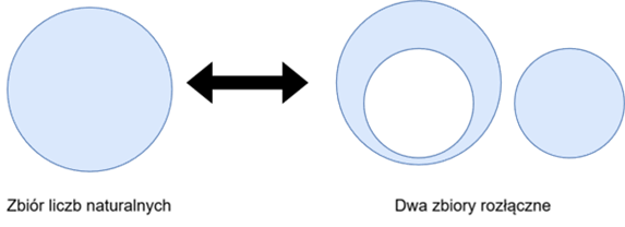
Fig. 1. Graphical representation of the concept of disjoint sets
These two sequences partition the set of natural numbers. This means that given two irrational numbers satisfying the relation stated in the theorem, we can split the entire set of natural numbers into two disjoint sets (Fig. 1).
The Beatty theorem is a fascinating observation in its own right - but in computer systems we run into a problem with irrational numbers. Real numbers - despite the fact that some programming languages use the words Real or Float for the real-number type - have little in common with actual real numbers. The fundamental problem is that we don’t have them, and presumably never will.
And here our journey would have abruptly ended, were it not for another theorem. The situation changed dramatically thanks to a mathematician - Aviezri Siegmund Fraenkel (1926), who specializes in combinatorial aspects of game theory.
In 1969 he presented the following theorem [2]. The starting point is a parameterized Beatty sequence:
\[ \mathcal{B}(\alpha ,\alpha ^{\prime }):= \left( \left\lfloor \frac{n-\alpha^{\prime }}{\alpha }\right\rfloor \right) _{n=1}^{\infty } \]
This single definition generates an entire family of sequences. The theorem always concerns a pair of its instances with different parameters: the sequence
\[ \mathcal{B}(\alpha ,\alpha ^{\prime }) \quad\text{and}\quad \mathcal{B}(\beta ,\beta ^{\prime }):= \left( \left\lfloor \frac{n-\beta^{\prime }}{\beta }\right\rfloor \right) _{n=1}^{\infty } \]
These sequences partition the set ℕ if and only if the following five conditions are satisfied:
1.
\[ 0<\alpha<1 \]
2.
\[ \alpha+\beta=1 \]
3.
\[ 0\leq \alpha +\alpha ^{\prime }\leq 1 \]
- If α is an irrational number, then:
\[ \alpha ^{\prime }+\beta ^{\prime }=0 \]
and
\[ k\alpha +\alpha ^{\prime }\not\in \mathbb{Z} \]
for
\[ 2\leq k\in \mathbb{N} \]
- If α is a rational number (let q∈N be the smallest number such that qα∈N), then
\[ \frac{1}{q}\leq \alpha +\alpha ^{\prime } \]
and
\[ \left\lceil q\alpha ^{\prime }\right\rceil +\left\lceil q\beta ^{\prime}\right\rceil =1 \]
And that is exactly what we need! We don’t have irrational numbers, but rational numbers understood as the ratio of two natural numbers are something a computer can handle just fine.
In our case, I first built prototype equations in Python, and then started looking for mathematical foundations that looked similar and could serve as well-documented equations backed by formal proofs. Proofs, of course, carried out by more experienced mathematicians. Modest as my skills were, they were enough to identify these two publications as relevant to my ideas.
This document does not include formal proofs. That is why I present here only the equations and theorems actually used in the system. For the formal proofs, I refer the reader to my scientific publications [3].
Algebra of Regular Time Series
Algebra - understood as a construct consisting of a defined set and defined operations on it - forms the basis for the declarative query language developed here. Throughout the rest of this work, when referring to “the Algebra” (without a further qualifier) I mean the Algebra of regular time series. When I want to refer to Relational Algebra, I will state the qualifier explicitly.
I proposed [3] the following definition of a regular time series (the so-called data model), along with the following operations and definitions.
✅ Note
By a data stream we understand an ordered pair S := (sn,∆) - where the first element is an ordered series of data and the second, denoted by the symbol delta, is the regular time interval between consecutive elements of the series.
We adopt a fixed indexing convention: stream indices run from zero, and element sn carries an implicit, default timestamp of (n+1)·∆. In other words - the first element of the stream appears after a full interval ∆ has elapsed since the stream’s creation. The timestamp is not carried within the tuple; it is derived from the position n and the rate ∆. It is precisely this differential data model that distinguishes the system from classical DSMS, where a stream is a multiset of pairs ⟨s,τ⟩ with a timestamp attached to every tuple.
A data series defined this way is referred to in the system as a data stream. Such a regularly flowing set of data passing through the system, usually described by a data schema, contains fields of various types. Each reading occurs at an equal time interval between consecutive measurements. This construction resembles a digital signal more than an irregular data stream - however, referring to it as a “stream” throughout the rest of the research will prove justified.
ℹ️ Info
Note:
The terms “stream” and “time series” are used interchangeably in this work and mean the same thing.
Formally, in the scientific literature a stream is denoted as a set of pairs (a,t) - where a denotes a tuple, and t denotes its moment of registration or occurrence.
A stream allows tuples whose time t coincides for different tuples. In the case of a time series, we distinguish two types of series - regular and irregular.
- For irregular series - a series is a sequence of tuples ordered in time - {at,tn}, where the time tn is unique in the set for each tuple.
- A regular time series, on the other hand, can be described by a sequence of tuples and a regular time interval between their occurrences - ({at},D) - and it is this latter definition that forms the basis for further operations in the system developed here.
The operations that can be performed on such a data set are defined as follows:
- interleaving and de-interleaving
- sum and difference
- sequence shift
- aggregation and serialization
The interleaving operation involves two different data streams.
We define it as follows:
\[ c_{n}=\left\{ \begin{array}{cc} b_{n-\left\lfloor n z \right\rfloor } & \left\lfloor n z \right\rfloor =\left\lfloor \left( n+1\right) z \right\rfloor \\ a_{\left\lfloor n z \right\rfloor } & \left\lfloor n z \right\rfloor \neq \left\lfloor \left( n+1\right) z \right\rfloor% \end{array}% \right. , z =\frac{\Delta _{b}}{\Delta _{a}+\Delta _{b}},\Delta _{c}=% \frac{\Delta _{a}\Delta _{b}}{\Delta _{a}+\Delta _{b}} \]
The arguments of the interleaving operation are two data streams A and B, each with its own data arrival rate. The result is an output stream C - with a new rate, different from the two source rates, determined by the formula above.
We denote the operation with the symbol #.
We define the de-interleaving operation by means of two operations.
1. Left-hand de-interleaving, producing stream A in the form:
\[ a_{n} = c_{n+ \left\lceil \frac{(n+1)\Delta _{a}}{\Delta _{b}} \right\rceil },\ \Delta _{a}=\frac{\Delta _{c}\Delta _{b}}{\left\vert \Delta _{c}-\Delta _{b}\right\vert } \]
- Right-hand de-interleaving, producing stream B in the form:
\[ b_{n} = c_{n+\left\lfloor \frac{n\Delta_{b}}{\Delta_{a}}\right\rfloor},\ \Delta_{b}=\frac{\Delta_{c}\Delta_{a}}{\left\vert \Delta_{c}-\Delta_{a}\right\vert } \]
We denote de-interleaving operations 1 and 2 with the symbols & and %.
The argument of the de-interleaving operation is an interleaved data stream together with a rational number specifying the arrival rate of the stream being extracted. The result of the operation is a data stream with the rate determined by the formula above.
The interleaving and de-interleaving operations are complementary. This means they resemble multiplication and division on the set of natural numbers. Multiplication yields a single result, whereas division sometimes leaves a remainder; what matters is also what we divide by, and in what order.
I defined the sum operation as follows:
\[ c_{n}=\left\{ \begin{array}{cc} a_{n}|b_{ \left\lfloor \frac{n\Delta_{a}}{\Delta_{b}} \right\rfloor } & \Delta_{a}\leq \Delta_{b} \\ a_{ \left\lfloor \frac {n\Delta_{b}}{\Delta_{a}} \right\rfloor }|b_{n} & \Delta_{a}>\Delta_{b} \end{array} \right. ,\Delta_{c}=\min \left( \Delta_{a},\Delta_{b}\right) \]
The faster stream dictates the rate of the result: each of its elements is joined (the symbol | denotes tuple concatenation) with the element occupying the co-indexed slot of the slower stream.
The difference, on the other hand, is described by the formula:
\[ a_{n}=\left\{ \begin{array}{cc} c_{n} & \Delta_{b}\geqslant \Delta_{a} \\ c_{\left\lceil \frac{n\Delta_{a}}{\Delta_{b}}\right\rceil } & \Delta_{b}<\Delta_{a} \end{array} \right. \]
We denote these operations with the symbols + and -.
Causal execution augments the mathematical stream S = (sn, ∆) with a logical origin OS ∈ ℕ and a startup tail WS ∈ ℕ. The logical origin is the index of the first record that exists at all; the tail is the number of subsequent slots for which an existing record is not yet ready. Neither kind of slot is a record: the engine inserts neither zeros nor all-null placeholders.
\[ \widehat{S} := \left((s_n,\Delta),O_S,W_S\right) \]
We define the shift as a read of an older index: output record \(n\) carries the contents of producer record \(n-m\). In the causal realization:
\[ O_{\tau_m(S)}=O_S+m, \qquad W_{\tau_m(S)}=\max(0,W_S-m), \qquad m\in\mathbb{N} \]
A shift neither discards source elements nor creates a prefix. It moves delay into the logical origin, while reading an older record can absorb part of the producer’s tail. The compiler reports both quantities as origin= and tail=. The runtime emits no records in any silent slot, of which there are origin + tail. Details: Tails, logical origins and operator observability.
I denote the shift operation with the symbol >.
The last operation within the defined algebra is the aggregation and serialization operation - abbreviated as Agse. Although it may look like two separate operations, I have defined a two-argument operator implementing the logic of a sliding data window. The first argument is the window’s hop, the second is its width. The hop is a natural number specifying by how much the sliding data window must be shifted over the stream. We assume that the source data stream is split with respect to the data schema, which modifies its arrival rate. The window width is an integer, non-zero. Negative width values reverse the order in which the resulting elements are created, mirror-image fashion. Positive values preserve the sequential character of the sliding data windows created.
I denote the Agse operation with the symbol @.
To summarize, the algebra underlying the declarative query language is as follows:
\[ A_{rql}::=((s_n,\Delta_s), (\#,\&,\%,+,-,>,@)) \]
where the first element of the pair defining the algebra is the data model (s_n - the data series, ∆_s - its regular time interval), and the second is the set of operations formally defined on this data model.
Formal Foundations and Proofs
In the chapter on the algebra of regular time series I presented a set of operators together with the equations describing them. I deliberately omitted formal proofs there - I wanted to first show what the system does before explaining why it is allowed to do so. This page fills that gap. Here I gather the formal skeleton of the algebra: the connection between the stream operators and covering-system theory, along with proofs of the theorems underlying the correctness and optimization of query plans.
ℹ️ Info
The entire construction below stays within a single domain - the rational numbers. This is not a stylistic choice. It is the whole point. Beatty’s theorem needs irrational numbers, which a computer does not have. Fraenkel’s theorem lets us descend to rational numbers. The proofs on this page show that the interleaving and de-interleaving operations are a special case of Beatty sequences satisfying Fraenkel’s postulates - and are therefore realizable using rational numbers alone.
Covering systems as the foundation
The literature on covering systems [4] belongs to combinatorics and cryptanalysis within number theory. The problem under consideration is how to determine a partition of the set of positive natural numbers. We say that two sequences partition the set of positive natural numbers if the sets formed from the elements of these sequences have an empty intersection, and their union forms the set of positive natural numbers.
The basis for these considerations is the parameterized Beatty sequence. In its general form it is written using the floor function:
\[ \mathcal{B}(\alpha ,\alpha ^{\prime }) := \left( \left\lfloor \frac{n-\alpha ^{\prime }}{\alpha }\right\rfloor \right) _{n=1}^{\infty } \]
This single definition generates an entire family of sequences. Partition results always concern a pair of its instances with different parameters: we write the pair as B(α, α′) and B(β, β′), where the second notation denotes the complementary term.
The parameters of this sequence have a clear geometric interpretation:
- α denotes the density of the sequence,
- 1/α denotes the slope,
- α′ denotes the offset,
- −α′/α denotes the y-intercept (the point where it crosses the y-axis).
The Beatty theorem guarantees a partition of the set for irrational numbers. The Fraenkel theorem is a generalization that - crucially for us - also allows rational numbers, provided five postulates are satisfied (quoted in the introductory chapter). An accessible proof of Fraenkel’s theorem can be found in K. O’Bryant’s paper “Fraenkel’s partition and Brown’s decomposition” [23].
The remainder of this page boils down to a single idea: showing that the stream operators are, in essence, machines generating Beatty sequences that partition (cover) the set of natural numbers.
Tools: floor and ceiling properties
The proofs rely almost exclusively on the floor function (⌊x⌋ - the integer part) and the ceiling function (⌈x⌉ - the smallest integer not less than x). I therefore first present a set of identities that will be used repeatedly. Let x ∈ ℝ, and let C denote an integer:
\[ \left\lfloor x\right\rfloor = \left\lceil x\right\rceil \iff x \in \mathbb{Z} \]
\[ \left\lfloor x\right\rfloor + 1 = \left\lceil x\right\rceil \iff x \in \mathbb{R} \setminus \mathbb{Z} \]
The second of these identities carries over directly to Beatty sequences themselves. The ceiling variant of the sequence, B′α(n) = ⌈nα⌉, is - for irrational α - merely a shifted version of the floor variant:
\[ B_{\alpha}^{\prime}(n) = \left\lceil n\alpha \right\rceil = \left\lfloor n\alpha \right\rfloor + 1 \]
In a true Beatty sequence α must be irrational, so nα is never an integer for any n > 0 - the premise of the second identity holds for every term, and the ceiling variant simply raises every term of the floor variant by exactly 1. For us, however, this is the case that does not exist inside a computer. In the rational domain, admitted only by Fraenkel’s theorem, nα is sometimes an integer, and then ⌈nα⌉ = ⌊nα⌋, so the shift by 1 disappears. The constant offset between the ceiling and the floor variant therefore ceases to hold globally and has to be settled term by term - which is exactly what the case analysis in part three of the proof of Theorem 2 (de-interleaving satisfies Fraenkel’s postulates) does, where gcd(a, b) decides which of the two cases applies.
\[ \left\lfloor x + C\right\rfloor = \left\lfloor x\right\rfloor + C \]
(the last identity holds for every C ∈ ℤ). Additionally, in analyzing the residue of the de-interleaving sequence we will use relationships tying the greatest common divisor (gcd) to the domain of the quotient a/b. For a, b ∈ ℕ>0:
\[ \operatorname{gcd}(a,b) = b \iff \frac{a}{b} \in \mathbb{N} \]
and otherwise:
\[ 1 \leq \operatorname{gcd}(a,b) \leq \min(a,b) \]
These two cases disjointly cover the entire domain of interest to us - which will let us carry out a proof “by cases.”
Operators in formal notation
The operators introduced in the query language have their formal counterparts. The table below ties the formal notation (used in the proofs) to the symbols found in the query language:
| Operation | Formal symbol | Symbol in the query language |
|---|---|---|
| Projection | π | field list after SELECT |
| Selection | σ | logical condition |
| Sum | Σ | + |
| Difference | δ | - |
| Interleaving | φ | # |
| De-interleaving and its complement | Θ, ∼Θ | & , % |
| Aggregation and serialization (AGSE) | Ψ | @ |
| Shift | τ | > |
For the proofs to be self-contained, I restate two definitions I will refer to directly.
Interleaving φ(A, B) produces an output stream whose successive tuples are determined by the rule:
\[ c_{n}= \left\{ \begin{array}{cc} b_{n-\left\lfloor n z \right\rfloor } & \left\lfloor n z \right\rfloor = \left\lfloor \left( n+1\right) z \right\rfloor \\ a_{\left\lfloor n z \right\rfloor } & \left\lfloor n z \right\rfloor \neq \left\lfloor \left( n+1\right) z \right\rfloor \end{array} \right. , \ z = \frac{\Delta _{b}}{\Delta _{a}+\Delta _{b}}, \ \Delta _{c}=\frac{\Delta _{a}\Delta _{b}}{\Delta _{a}+\Delta _{b}} \]
De-interleaving is defined by two complementary formulas - operator Θ, which recovers the original stream, and operator ∼Θ, which determines the “remainder” of the de-interleaving:
\[ a_{n} = c_{n+ \left\lceil \frac{(n+1)\Delta _{a}}{\Delta _{b}} \right\rceil },\ \Delta _{a}=\frac{\Delta _{c}\Delta _{b}}{\left\vert \Delta _{c}-\Delta _{b}\right\vert } \]
\[ b_{n} = c_{n+\left\lfloor \frac{n\Delta_{b}}{\Delta_{a}}\right\rfloor},\ \Delta_{b}=\frac{\Delta_{c}\Delta_{a}}{\left\vert \Delta_{c}-\Delta_{a}\right\vert } \]
Theorem 1: interleaving guarantees set coverage
✅ Note
Theorem. The interleaving operation guarantees sequential coverage of both index sets of the data streams that are its arguments: every element of stream A and every element of stream B is selected exactly once, in order, without gaps and without repetition.
Proof. Since 0 < z < 1, the increment
\[ d_{n} := \left\lfloor \left( n+1\right) z \right\rfloor - \left\lfloor n z \right\rfloor \]
equals 0 or 1 for every n ≥ 0. The interleaving equation selects an element of stream B exactly at those steps where dn = 0 (the equality branch), and an element of stream A exactly at steps where dn = 1.
Consider the selection index for sequence B: xn = n − ⌊nz⌋. In a single step, xn+1 − xn = 1 − dn: the index increases by exactly 1 at every step selecting from B, and otherwise remains unchanged. So if n < n′ are two consecutive steps selecting from B, then xn′ = xn + 1. The first step selecting from B is n = 0, since 0 < z < 1 implies ⌊0⌋ = ⌊z⌋ = 0, i.e. d0 = 0, and x0 = 0. Selections from sequence B therefore use indices 0, 1, 2, … in order, without gaps or repetitions.
Symmetrically: the selection index for sequence A, i.e. ⌊nz⌋, increases by exactly 1 at every step selecting from A (dn = 1), and otherwise remains unchanged; at the first such step its value is 0 (all earlier steps have d = 0). The elements of sequence A are therefore also selected exactly once each, in order. ∎
Theorem 2: de-interleaving satisfies Fraenkel’s postulates
This is the central theorem of this page. It proves that the two sequences describing the de-interleaving operation are a special case of Beatty sequences satisfying the postulates of Fraenkel’s theorem for rational numbers. Without this theorem, the whole system remains merely a promise.
✅ Note
Theorem. Let a, b ∈ ℕ>0 represent the rational ratio of the rates of the component streams, ∆a/∆b = a/b. Both tuple-selection sequences describing the de-interleaving operation are - up to the index alignment shown in the proof - a special case of Beatty sequences satisfying the postulates of Fraenkel’s theorem for rational parameters. Consequently they partition the set ℕ₀ := ℕ ∪ {0}, i.e. the index set of the interleaved stream, and de-interleaving exactly inverts interleaving using rational-number arithmetic alone.
Proof - part one (reduction to Beatty form). The tuple-selection sequence for the de-interleaving residue (operator ∼Θ) has the form:
\[ \left( n + \left\lfloor \frac{nb}{a} \right\rfloor \right) _{n=0}^{\infty } \]
Its initial term (n = 0) equals 0; the terms for n ≥ 1 form the Beatty part. For n ∈ ℕ, by the property ⌊x + C⌋ = ⌊x⌋ + C, we have n + ⌊nb/a⌋ = ⌊n + nb/a⌋, so we seek α, α′ such that:
\[ \left( \left\lfloor \frac{n-\alpha ^{\prime }}{\alpha }\right\rfloor \right) _{n=1}^{\infty } = \left( \left\lfloor n\frac{a + b}{a} \right\rfloor \right) _{n=1}^{\infty } \]
Reading off the slope and the offset: with a shift of α′ = 0 we obtain α = a/(a+b), and the selection sequence restricted to n ≥ 1 is exactly:
\[ \mathcal{B}\!\left( \frac{a}{a + b}, 0 \right) = \left( \left\lfloor n\frac{a + b}{a} \right\rfloor \right) _{n=1}^{\infty } \]
Proof - part two (verifying the five postulates and determining the residue). We check the postulates of Fraenkel’s theorem in turn for α = a/(a+b), α′ = 0:
- The value α = a/(a+b) for a, b > 0 is greater than zero and less than one.
- The condition α + β = 1 is satisfied for β = b/(a+b).
- For α′ = 0 the postulate is equivalent to postulate 1.
- The postulate is vacuous, since α is a rational number.
- The smallest number q for which qα ∈ ℕ is q = (a+b)/gcd(a,b); then the condition 1/q ≤ α + α′ = α is satisfied, and the condition ⌈qα′⌉ + ⌈qβ′⌉ = 1 with α′ = 0 forces ⌈qβ′⌉ = 1, i.e. 0 < β′ ≤ gcd(a,b)/(a+b). Every admissible value generates the same sequence (the complement of the sequence B(a/(a+b), 0) in ℕ is unique); we take β′ = gcd(a,b)/(a+b).
The sequence complementing B(a/(a+b), 0) in the sense of Fraenkel’s postulates is therefore:
\[ \mathcal{B}\!\left( \frac{b}{a + b}, \frac{\operatorname{gcd}(a, b)}{a + b} \right) \]
After reindexing n ↦ n + 1, so that it runs from n = 0 - matching the selection sequences in the definition of de-interleaving - it takes the form:
\[ \left( \left\lfloor \frac{(n + 1) - \frac{\operatorname{gcd}(a,b)}{a+b}}{\frac{b}{a+b}} \right\rfloor \right) _{n=0}^{\infty } \]
Expanding the above expression:
\[ \left\lfloor \frac{(n + 1) - \frac{\operatorname{gcd}(a,b)}{a+b}}{\frac{b}{a+b}} \right\rfloor = \left\lfloor n\frac{a}{b} + n + \frac{a}{b} + 1 - \frac{\operatorname{gcd}(a, b)}{b} \right\rfloor \]
Comparing this - term by term for n ≥ 0 - with the tuple-selection sequence of the recovered stream (operator Θ):
\[ \left( n + \left\lceil \frac{(n + 1)a}{b} \right\rceil \right) _{n=0}^{\infty } \]
and factoring out the integer part n + 1 via the property ⌊x + C⌋ = ⌊x⌋ + C, the claim reduces (after substituting n for n + 1, so that n ranges over ℕ>0) to the identity:
\[ \left\lfloor n\frac{a}{b} - \frac{\operatorname{gcd}(a, b)}{b} \right\rfloor + 1 = \left\lceil n\frac{a}{b} \right\rceil ,\quad n \in \mathbb{N}_{>0} \]
Proof - part three (case analysis). Using the properties of the coefficient gcd(a, b), we consider two disjoint cases covering the entire domain.
Case 1: gcd(a, b) = b, i.e. a/b ∈ ℕ. Then n·a/b ∈ ℕ, so by the identity ⌊x⌋ = ⌈x⌉ ⟺ x ∈ ℤ we have ⌈n·a/b⌉ = ⌊n·a/b⌋, and by ⌊x + C⌋ = ⌊x⌋ + C:
\[ \left\lfloor n\frac{a}{b} - 1 \right\rfloor + 1 = \left\lfloor n\frac{a}{b} \right\rfloor \]
Both sides of the identity being proved coincide.
Case 2: b ∤ a, i.e. 1 ≤ gcd(a, b) < b and 0 < gcd(a,b)/b < 1.
If n·a/b ∉ ℤ, then by ⌊x⌋ + 1 = ⌈x⌉ ⟺ x ∈ ℝ ∖ ℤ we have ⌈n·a/b⌉ = ⌊n·a/b⌋ + 1. The fractional part of n·a/b is a nonzero multiple of gcd(a,b)/b, and hence at least gcd(a,b)/b; subtracting gcd(a,b)/b from n·a/b therefore cannot drop below the integer ⌊n·a/b⌋, whence:
\[ \left\lfloor n\frac{a}{b} - \frac{\operatorname{gcd}(a, b)}{b} \right\rfloor = \left\lfloor n\frac{a}{b} \right\rfloor \]
and the identity being proved holds.
If n·a/b ∈ ℤ, then ⌈n·a/b⌉ = n·a/b, and since 0 < gcd(a,b)/b < 1:
\[ \left\lfloor n\frac{a}{b} - \frac{\operatorname{gcd}(a, b)}{b} \right\rfloor = n\frac{a}{b} - 1 \]
which again gives the identity being proved.
Both selection sequences describing the de-interleaving operation are therefore - up to the unit reindexing from part two - Beatty sequences satisfying Fraenkel’s postulates for rational parameters: the pair B(a/(a+b), 0) and B(b/(a+b), gcd(a,b)/(a+b)) partitions the set ℕ, and together with the initial residue term 0 from part one - the set ℕ₀, the full index set of the interleaved stream. The recovered stream and the residue are therefore exact. ∎
✅ Note
Corollary (exact invertibility over the rationals). For streams with rational rates, the operators Θ and ∼Θ recover the component streams of φ(A, B) exactly (bit for bit): no tuple is lost, duplicated, or reordered relative to its component stream. The pair (φ; Θ, ∼Θ) therefore behaves like multiplication and division, and the pair (Σ; δ) like addition and subtraction, on the set of regular time series.
⚠️ Warning
The practical takeaway from this proof: the implementation must never leave the domain of rational numbers, not even momentarily. An implicit cast of an intermediate result to a floating-point number breaks the assumptions of the theorem above. Materialization into floating-point form must be deferred until an explicit application of the floor or ceiling operation.
Operator properties used in optimization
Based on the algebra presented, a number of properties of data streams can be shown. They have direct application in the data-management system - during query-plan optimization and result interpretation.
Disruption of event ordering
✅ Note
Theorem. The order of elements in a stream does not reflect the actual order in which the elements occurred in the real world.
Proof (by counterexample). Consider two streams:
Alpha(char),2:   {1,2,3,4,5,6,...}
Epsilon(char),3: {a,b,c,d,e,f,...}
The expression φ(Epsilon, Alpha) produces the output stream:
Tau(char),6/5: {1,2,a,3,b,4,5,c,6,d,...}
In stream Tau, the tuple labeled c occurs after the tuple labeled 5. Yet tuple c appears in stream Epsilon at second 9, while tuple 5 appears in stream Alpha at second 10. The natural order of events has been violated in the resulting stream. Conclusion: when analyzing time embedded in streams, applying the de-interleaving operation is necessary to recover the original form of the data streams. ∎
Commutativity of summation
✅ Note
Theorem. The stream-summation operation, disregarding attribute order, is commutative.
Proof. Assume ∆a ≤ ∆b; the opposite case is symmetric. The first case of the sum definition gives, as the n-th element of stream Σ(A, B), the tuple:
\[ c_{n} = \left( a_{n},\ b_{\left\lfloor n\Delta_{a}/\Delta_{b} \right\rfloor} \right) \]
whereas for Σ(B, A) the roles of the arguments are swapped, and its second case applies (or, at ∆a = ∆b, its first), giving as the n-th element:
\[ c_{n} = \left( b_{\left\lfloor n\Delta_{a}/\Delta_{b} \right\rfloor},\ a_{n} \right) \]
Both streams carry ∆c = ∆a. They therefore coincide up to the order of the joined attributes. ∎
Interleaving alignment method
The interleaving operation is not commutative in general: since 0 < z < 1, at n = 0 the equality branch of the interleaving definition always applies, so the stream φ(A, B) begins with element b₀, while the stream φ(B, A) begins with element a₀. Interleaving is, however, equivariant with respect to time shifts matched to the streams’ rates - which is valuable for query-plan optimization.
In the causal realization a stream has the form \(\widehat{S}=((s_n,\Delta),W_S)\), where \(W_S\) is its startup tail. We define conversion of a producer’s tail into output slots as:
\[ \operatorname{conv}(w,\Delta_s,\Delta_o):= \left\lceil\frac{w\Delta_s}{\Delta_o}\right\rceil \]
The tail of an interleave with interval \(\Delta_c=\Delta_a\Delta_b/(\Delta_a+\Delta_b)\) follows directly from the operator definition, without going through a single phase term.
Record \(i\) of \(\varphi(A,B)\) carries the content of record \(j(i)\) of exactly one component - the one the interleave definition selects in slot \(i\). Write \(\Delta_{s(i)}\) and \(W_{s(i)}\) for the interval and tail of the selected component. Record \(j(i)\) is determined at time \(\bigl(j(i)+1+W_{s(i)}\bigr)\Delta_{s(i)}\), while consumer slot \(i\) ends at \((i+1+W)\Delta_c\). The causality condition for every \(i\) is:
\[ W\ge \left\lceil\frac{\bigl(j(i)+1+W_{s(i)}\bigr)\Delta_{s(i)}}{\Delta_c}\right\rceil -1-i \]
Let \(\Delta_a/\Delta_b=p/q\), where \(p,q\in\mathbb{N}_{>0}\) and \(\gcd(p,q)=1\). Both the component selection and the residue determining \(j(i)\) repeat with period \(p+q\), so the maximum of the right-hand side over one period is the maximum over all records:
\[ W_{\varphi(A,B)} =\max_{0\le i<p+q}\left( \left\lceil\frac{\bigl(j(i)+1+W_{s(i)}\bigr)\Delta_{s(i)}}{\Delta_c}\right\rceil -1-i \right) \]
The formula is exact: it neither overshoots nor undershoots the event-model bound for any node. The period scan starts at zero - the logical origin shifts the consumer index and the component index by the same amount, so the window \([0,,p+q)\) yields the same value as any shifted window.
The earlier closed form
\[ W_{\varphi(A,B)} =\max\left( \operatorname{conv}(W_A,\Delta_a,\Delta_c), \operatorname{conv}(W_B,\Delta_b,\Delta_c) +H_{a,b} \right), \qquad H_{a,b}=\left\lceil\frac{p+q-1}{p}\right\rceil \]
protected the worst read phase of the second argument, but did not check whether that phase actually falls on the record that waits longest - hence it overshot the tail by one slot for some nodes. It survives in the implementation as the fallback for \(p+q\) above the scan threshold (kHashPhaseScanLimit in SOperations.hpp): overshooting costs one slot of latency, whereas undershooting would mean emitting a record before its dependency is determined. Tail slots are not records.
The shift \(\tau_m\) does not change the emitted record sequence, but it does change the index at which that sequence appears: record \(n\) carries the content of record \(n-m\). Records with an index below \(O_S+m\) have no definition, hence
\[ O_{\tau_m(S)}=O_S+m, \qquad W_{\tau_m(S)}=\max\left(0,;W_S-m\right) \]
The tail decreases: record \(n-m\) is older than the current one and therefore all the more available - the slot deficit is \(W_S-m\) and is constant. Details and measurement: Tails, logical origins and operator observability.
✅ Note
Theorem (R1, commuting a shift with an interleave). If numbers i, k ∈ ℕ are chosen such that i·∆a = k·∆b (both arguments shifted by the same amount of time), then interleaving the shifted streams and the interleaving of the original streams shifted by the sum of these numbers have the same record sequence, the same interval and the same logical origin. Their tails satisfy an inequality - the factored side is never the later one.
Formally, with \(L:=i+k\):
\[ \operatorname{Obs}\Bigl(\varphi\bigl(\tau_{i}(A),\tau_{k}(B)\bigr)\Bigr) =\operatorname{Obs}\Bigl(\tau_{i+k}\bigl(\varphi(A,B)\bigr)\Bigr), \qquad i\Delta_{a}=k\Delta_{b},\quad i,k\in\mathbb{N} \]
\[ W_{\mathrm{RHS}}=\max\left(0,;W_{\varphi(A,B)}-L\right)\le W_{\mathrm{LHS}} \]
where \(\operatorname{Obs}\) is the value part of the observation (interval, logical origin, record sequence with its NULL map, descriptor, gap trace, materialization policy) - see Tails, logical origins and operator observability.
Proof.
Interval. Both sides arise from the same interleave, so both have \(\Delta_c=\Delta_a\Delta_b/(\Delta_a+\Delta_b)\).
Auxiliary step. From i·∆a = k·∆b it follows that
\[ \frac{i\Delta_a}{\Delta_c} =\frac{i\Delta_a(\Delta_a+\Delta_b)}{\Delta_a\Delta_b} =\frac{i\Delta_a}{\Delta_b}+i =k+i =L\in\mathbb{N}, \]
and symmetrically \(k\Delta_b/\Delta_c=L\). Shifting each argument by its own number of slots therefore corresponds to the same number \(L\) of result slots.
Record sequence and logical origin. Within one period the interleave takes \(i\) records from A and \(k\) records from B, filling exactly \(L=i+k\) slots of C. Shifting A by \(i\) and B by \(k\) therefore moves the mapping threshold of both components by exactly \(L\) result slots without changing their relative phase: \(O_{\mathrm{LHS}}=O_{\varphi(A,B)}+L=O_{\mathrm{RHS}}\). The content of a record at a given logical index is the same on both sides, because the choice of component depends only on phase, which is unchanged.
Tails. Let \(s(n)\in\{A,B\}\) denote the component selected in phase \(n\), and \(j(n)\) its index. Write the shifts as \(t_A=i\) and \(t_B=k\). After shifting, the component tail is \(W_s^{\prime}=\max(0,W_s-t_s)\ge W_s-t_s\). The intervals and the choice of component and its index in each interleave phase remain unchanged. Let \(R_n\) be the availability requirement from the phase formula above for tails \(W_A,W_B\), and \(R_n^{\prime}\) the requirement for \(W_A^{\prime},W_B^{\prime}\). The auxiliary step gives \(t_s\Delta_s/\Delta_c=L\in\mathbb{N}\) for both components. Monotonicity of the ceiling and its compatibility with shifts by the integer \(L\) give, in every phase:
\[ \begin{aligned} R_n^{\prime} &=\left\lceil \frac{(j(n)+1+W_{s(n)}^{\prime})\Delta_{s(n)}}{\Delta_c} \right\rceil-1-n\\ &\ge\left\lceil \frac{(j(n)+1+W_{s(n)}-t_{s(n)})\Delta_{s(n)}}{\Delta_c} \right\rceil-1-n =R_n-L. \end{aligned} \]
We take the maximum over the same full period \(p+q\), since the shifts do not change the interval ratio. Using nonnegativity of tails as well, we obtain:
\[ W_{\mathrm{LHS}} \ge\max\left(0,\max_{0\le n<p+q}R_n-L\right) =\max\left(0,W_{\varphi(A,B)}-L\right) =W_{\mathrm{RHS}}. \]
Above the scan limit, the engine uses the \(O(1)\) fallback bound described earlier. For that bound, the same inequality follows from monotonicity of both \(\operatorname{conv}\) terms: a matched shift reduces each by at most \(L\), while the \(H_{a,b}\) term remains unchanged. Both sides use the same calculation variant because their intervals do not change. The fallback bound need not equal the exact phase maximum. ∎
⚠️ Scope of the theorem
Equality of tails does not hold. Counterexample: \(\Delta_a=1/10\), \(\Delta_b=1/5\), \(W_A=W_B=0\), \(H_{a,b}=2\), \(i=2\), \(k=1\), \(L=3\). Then \(W_{\mathrm{LHS}}=2\) while \(W_{\mathrm{RHS}}=\max(0,2-3)=0\). The unfactored side reads its components after their own shift, so it waits longer for the same content; the factored side reads it directly from the interleave.
Practical consequence: the rewrite rule \(\varphi(\tau_i(A),\tau_k(B))\to\tau_{i+k}(\varphi(A,B))\) is a latency optimization, not a neutral rewrite. It preserves the entire value part of the observation and never emits a record before its dependencies are determined, but the result is ready sooner.
Previously both sides had the same tail solely because the realization of \(\tau_m\) overestimated its own tail by \(\min(W_S,m)\). The overestimate was removed by addressing the producer with a logical index instead of a relative offset. Regressions guarding this scope:
it_r1_identity_nulls,it_optimizer_ablation-factor-name-collision-semantic.
In the compiler, additional invariants preserve public stream field names, null value maps, and the materialization policy.
Why this matters
The theorems presented are not formalism for its own sake. Each of them plays a concrete role in the working system:
- Theorems 1 and 2 guarantee that the pairs of operations interleaving/de-interleaving and sum/difference are complementary - data is neither lost nor duplicated in an uncontrolled way. They are what allow us to treat these operations like multiplication/division and addition/subtraction on the set of regular time series.
- Theorem 2 in particular proves that the entire construction can be realized using rational numbers alone - and thus deterministically and exactly on a computer. This is the condition without which RetractorDB could not exist.
- The theorems on operator properties (commutativity of summation, interleaving alignment, ordering disruption) provide rewrite rules for stream expressions. The query-plan optimizer uses them to transform plans into cheaper-to-execute forms without changing the result.
The branch of mathematics in which these equations are situated is the theory of covering systems [4] within number theory. I presented the full formalism along with a complete set of proofs in the paper A Deterministic Method for Processing Data Sequences [3].
ℹ️ Info
A numerical verification of the equations above - Python prototypes operating on rational numbers (the
Fractionlibrary) - can be found on the Model Implementation page and in the repository github.com/michalwidera/equations.
Tails, logical origins and operator observability
A causal realization extends a stream \(S=(s_n,\Delta_S)\) with two integer quantities, not one. The distinction matters: they answer different questions and behave differently under plan rewrites.
| Quantity | Question | Meaning |
|---|---|---|
| logical origin \(O_S\) | which record is missing? | index of the first record that exists at all; records with a lower index have no definition, because they would reach before the start of the source stream |
| startup tail \(W_S\) | when is a record ready? | record \(n\) is emitted at time \((n+1+W_S)\Delta_S\) |
Neither is a prefix of zeros or of all-null records. The boundary principle holds unchanged: NULL is a data value, never a placeholder. The number of initial slots in which the stream stays silent is \(O_S+W_S\) - and only that sum was visible before the two quantities were separated.
The logical index is the currency of every mapping between streams. A stream with a non-zero \(O_S\) has no earlier records, so its physical record 0 carries logical index \(O_S\); the conversion to a buffer offset is performed solely by dataModel::fetchForward().
Operator audit
In the table, “own tail” is the delay required by the operator beyond producer availability. Producer tails are converted to result slots beforehand.
| Operator | Source index or bound | Logical origin | Own tail | Test |
|---|---|---|---|---|
projection / PUSH_STREAM | current tuple | \(O_S\) | 0 | ut_compiler |
shift >N | record \(n-N\) | \(O_S+N\) | \(-N\), see below | ut_compiler, ut_h10aGate |
sum + | current co-indexed tuples | mapping threshold | 0 | ut_compiler |
interleave # | record \(j(i)\) of the component selected in slot \(i\) | mapping threshold | formula below | deinterleave_roundtrip, ut_h10aGate |
left de-interleave & (DIV) | \(n+\lceil(n+1)\Delta_a/\Delta_b\rceil\) | mapping threshold | phase formula below | deinterleave_roundtrip, ut_h10aGate |
right de-interleave % (MOD) | \(n+\lfloor n\Delta_b/\Delta_a\rfloor\) | mapping threshold | phase formula below | deinterleave_roundtrip, ut_h10aGate |
difference C-Delta | \(\lceil n\Delta/\Delta_C\rceil\) | mapping threshold | phase formula below | it_k19_boundaries, ut_h10aGate |
AGSE @(k,L) | fields from \(nk-(\lvert L\rvert-1)\) to \(nk\) | formula below | formula below | agse1, agse2, agse3, it_k19_boundaries, ut_h10aGate |
sumc, avgc, minc, maxc | current full tuple | \(O_S\) | 0 | ut_dataModel, it_k19_boundaries |
“Mapping threshold” is the smallest index \(n\) from which every later record maps onto existing component records. It is not “the first index with complete dependencies”: with an interleave of components having different origins, record 0 may be complete while record 1 is not. A stream is a sequence of records, not a set with holes - the boundary principle forbids filling a hole with NULL - so the logical origin is the first index with no remaining gap. All record-to-record mappings are non-decreasing, so such an index exists and is unique.
The difference operator takes a target interval \(\Delta\) that may not be smaller than the source interval \(\Delta_C\). For the ratio \(r=\Delta/\Delta_C=p/q\) the maximum phase lead of the index \(\lceil nr\rceil\) is \((q-1)/q\).
Tails of phase operators
Difference and both de-interleaves use one availability rule. Let \(r=\Delta_{out}/\Delta_{src}\), let \(W_S\) be the source tail, and let \(e_{max}\) be the largest phase lead reached by the index mapping. Then:
\[ W_{out}=\max\left(0, \left\lceil\frac{e_{max}+W_S+1}{r}\right\rceil-1 \right) \]
For difference, \(e_{max}=(q-1)/q\), where \(q\) is the denominator of the reduced ratio \(r\). For left de-interleave, with \(\Delta_{out}/\Delta_{other}=a/b\), the value is \(e_{max}=(a+b-1)/b\). For right de-interleave, \(e_{max}=0\). In particular, left de-interleave does not unconditionally add one slot: for an integral ratio, its own tail can be zero.
The interleave tail
The interleave is the only operator whose tail does not decompose into “converted producer tails plus an own constant”. Record \(i\) carries the content of record \(j(i)\) of just one component - the one the operator definition selects in slot \(i\) - so the required latency depends on which component, and which of its phases, a given slot falls on:
\[ W_{\#} =\max_{0\le i<p+q}\left( \left\lceil\frac{\bigl(j(i)+1+W_{s(i)}\bigr)\Delta_{s(i)}}{\Delta_c}\right\rceil -1-i \right), \qquad \frac{\Delta_a}{\Delta_b}=\frac{p}{q},\quad \gcd(p,q)=1 \]
The component selection and the phase repeat with period \(p+q\), so the maximum over one period is the maximum over all records; the logical origin shifts both indices equally and does not change the result. The formula is exact. For periods exceeding kHashPhaseScanLimit, a safe closed form protects the worst read phase. It may delay emission, but it cannot allow a record to be emitted before its dependencies are available.
The shift \(\tau_N\)
Record \(n\) carries the content of producer record \(n-N\). Hence both quantities:
\[ O_{\tau_N(S)}=O_S+N, \qquad W_{\tau_N(S)}=\max\left(0,;W_S-N\right) \]
The tail decreases, it does not grow. Record \(n-N\) is older than the current one, so it is available all the more readily: the deficit of slot \(n\) is \((n-N+1+W_S)-(n+1)=W_S-N\) and is constant, independent of \(n\). The shift therefore moves silence from the tail into the logical origin, and additionally absorbs the producer tail whenever \(N\ge W_S\).
The sum \(O+W\) is not invariant here: for \(N<W_S\) it equals \(W_S\), whereas the realization from before the separation gave \(W_S+N\). That earlier realization overestimated the tail by \(\min(W_S,N)\); the overestimate was removed by addressing the producer with a logical index instead of a relative offset.
The full AGSE window
The window is stamped by the interval end: record \(n\) spans flattened source positions from \(nk-(\lvert L\rvert-1)\) to \(nk\). Its newest field therefore lies exactly at position \(nk\), and the window’s logical index denotes the same instant as the source’s logical index - joining a window with its own source (a FIR pipeline) does not lead the signal.
The price of the convention is that for small \(n\) the window would reach before the start of the source. Those records are not produced. Let the source have \(F\) fields and logical origin \(O_S\); requiring the whole window to fit gives
\[ O_{\operatorname{AGSE}} =\left\lceil\frac{O_S F+\lvert L\rvert-1}{k}\right\rceil \]
Availability is governed by the newest field, which lies in record \(\lfloor nk/F\rfloor\). Substituting \(r_n=(nk)\bmod F\), the availability condition for every \(n\) becomes \(W\ge\bigl(F(1+W_S)-r_n\bigr)/k-1\). The residues \(r_n\) run through multiples of \(\gcd(F,k)\) periodically, so the minimum \(r_n=0\) is attained regardless of the index at which the stream starts. Hence
\[ W_{\operatorname{AGSE}} =\left\lceil\frac{(1+W_S)F}{k}\right\rceil-1 \]
The phase term \(P_{F,k,L}=\lfloor(\lvert L\rvert-1)/g\rfloor,g\), present in the form used before the re-stamping, disappeared from the tail: the window span is not waiting but undefinedness, and moved wholly into the logical origin. The sum \(O+W\) describes the same silence as before.
A positive width preserves the historical RetractorDB convention - the newest field comes first; a negative width mirrors it, giving arrival order.
Source history capacity has no closed form here. The backward distance at the moment record \(n\) is emitted,
\[ \left\lfloor\frac{(n+1+W)k}{F}\right\rfloor-W_S-1 ;-; \left\lfloor\frac{nk-\lvert L\rvert+1}{F}\right\rfloor, \]
is periodic with period \(F/\gcd(F,k)\) output slots, so the maximum is computed exactly, by scanning one full period from \(O_{\operatorname{AGSE}}\). A closed form would be guesswork here, and underestimating means reading outside history, not merely one slot of delay. A declared source has one record armed when the storage is opened plus a zero prefetch, so its capacity bound contains two extra records. Capacity is a property of execution, not part of the result.
The observability relation
Stream observation splits into two parts, because plan rewrites preserve them to different degrees.
Value part - preserved by rewrites exactly:
\[ \operatorname{Obs}(S) =\left(\Delta_S,O_S,D_S,(s_n,N_n)_{n\ge O_S},G_S,M_S\right) \]
where:
- \(O_S\) is the logical origin, the index of the first record;
- \(D_S\) is the public descriptor and field-name order;
- \(N_n\) is the record’s
NULLmap - a trueNULLremains a data value and is carried through AGSE; - \(G_S\) is the gap trace; detection currently works for declarations, while computed streams have \(G_S=\varnothing\);
- \(M_S\) describes the materialization policy (
DEFAULT,MEMORY,VOLATILEand the remaining storage kinds).
Latency part - the tail \(W_S\) - carries a weaker guarantee:
a plan rewrite never increases \(W_S\) and never emits a record before its dependencies are determined; it may, however, decrease \(W_S\).
The split is not a formality. The \(R_1\) factoring (\(\varphi(\tau_i(A),\tau_k(B))\to\tau_{i+k}(\varphi(A,B))\)) preserves the whole value part but shortens the tail: the factored form reads content directly from the interleave, whereas the unfactored form reads components only after their own shift. Rationale: Formal foundations and proofs, theorem on commuting a shift with an interleave. Regressions: it_r1_identity_nulls, it_optimizer_ablation-factor-name-collision-semantic.
Changing any component of the value part changes the observable artifact. In particular, enabling gap propagation for computed streams in the future requires a versioned semantic change.
A read outside available history internally returns an all-null record as a failsafe. A correctly compiled plan never materializes it: logicalOrigin skips slots without a definition, startupLatency skips slots not yet determined, and the history capacity retains every required index. The it_k19_boundaries test distinguishes this case from a genuine NULL located inside a full window. Since 23 September 2026 the convention holds along the whole read path: storage::read() and storage::revRead() report a missing record through a separate status and also set an all-null pattern, so a reducer absorbs such a record instead of folding zeros out of it (→ Files).
The operator formulas in this chapter are enforced on every commit: boundaries and observability by it_k19_boundaries, history depths by it_k24_capacity, and agreement of logical origin and tail for all canonical operator classes and their compositions by the ut_h10aGate unit test.
Algebraic Expressions
The defined algebra entails the possibility of defining algebraic expressions. Typical algebraic expressions over the set of rational numbers are material covered in elementary school. Algebraic expressions in RetractorDB occur in two forms. In the field list of the SELECT command, we have the typical expressions familiar from school. In the argument list of the SELECT command’s FROM clause, we have an algebraic expression built on the newly defined algebra.
This means that in the field list after the SELECT clause, the plus operator means one thing, while in the FROM clause it means something else entirely. An innocent-looking query from the definition combines two entirely different worlds and concepts: one, an algebra based on numbers; the other, based on regular time series.
Example. As an example, we present an algebraic expression built over the set of regular time series (hereafter called streams). Assume the existence of two streams: A(a1 int, a2 int),1 and B(b1 int),½ - where,
- A denotes a stream containing, in each record, two fields of type int - a1 and a2 - arriving once per second, and
- B contains, in each record, a field of type int named b1 arriving twice per second.
The algebraic expression C=A+B creates a data stream with fields C(a1 int, a2 int, b1 int),½.
To interleave a data stream, sets A and B should have the same data schema. Let’s assume, then, that there is a stream D(d1 int),1 - arriving, like stream A, once per second.
The algebraic expression E=B#D creates the stream: E(e1 int),⅓. The rate ⅓ comes from the formula (1*½)/(1+½). You will find this formula in the definition of the interleaving operation.
For streams defined this way, the following expression is still valid:
F=((B#D)+A)>2
And such expressions may appear as valid, with respect to the developed time-series algebra, in the body of a query.
Further examples
Continuing with the streams defined above, A(a1 int, a2 int),1, B(b1 int),½ and D(d1 int),1, and the output streams C=A+B and E=B#D - below is a further set of valid algebraic expressions. Equivalents of all these expressions appear in FROM clauses of queries in the system’s integration tests, and are verified on every build of the project.
Interleaving the result of an interleave:
G=E#D
Stream E has rate ⅓, stream D has rate 1, both share the same schema with a single int field. The interleaving formula gives a rate of (⅓·1)/(⅓+1)=¼, so G(g1 int),¼. The result of one operation is a fully valid stream and can be the argument of the next one.
Sum of three streams:
H=A+B+D
Summation joins tuples, so the result schema is the concatenation of the schemas, and the rate is dictated by the fastest component: H(a1 int, a2 int, b1 int, d1 int),½.
Sum with a shifted component, and a shift of an interleaving argument:
I=D+((A+B)>1)
J=(B>1)#D
Shifting a sequence does not change the stream’s rate - it only changes data access by a given number of samples. Therefore I has rate min(1,½)=½, and J - just like E - has rate ⅓.
De-interleaving:
K=E&1
L=E%½
The right-hand argument of the de-interleaving operators is a rational number, not a stream. Substituting into the de-interleaving formulas: K has rate (⅓·1)/|⅓−1|=½ - left-hand de-interleaving recovers stream B from the interleave E. Similarly L has rate (⅓·½)/|⅓−½|=1 - right-hand de-interleaving recovers stream D. De-interleaving is the inverse of interleaving, just as division is the inverse of multiplication.
Difference:
M=C-1
Difference is the inverse operation to sum - it extracts, from the joined stream C, the component indicated by the rational number on the right-hand side of the operator.
Aggregation and serialization:
N=A@(1,4)
P=A@(1,-4)
R=A@(2,2)
S=(A@(2,2))@(1,1)
N creates a sliding window of width 4 shifted by one element, P - thanks to its negative width - builds the same windows mirror-imaged, R creates disjoint windows (hop equal to the width). Expression S shows that the result of an Agse operation can be the argument of another Agse operation.
All of the above forms can be combined into arbitrarily complex expressions - like F=((B#D)+A)>2 from the example above - as long as the data schemas of the arguments satisfy the requirements of the respective operations.
Coverage of examples in integration tests
Each of the expression forms cited has a counterpart in the RetractorDB repository’s shared test/IntegrationTest directory, executed on every project build:
| Expression from this chapter | Form in the test | Integration test |
|---|---|---|
| C=A+B (sum) | s1+s2, core0+core1 | IntegrationTest/issue167_dedup_positive, IntegrationTest/Data (all-operators) |
| E=B#D (interleaving) | core0#core1 | IntegrationTest/operations, IntegrationTest/Data (all-operators) |
| G=E#D (cascaded interleaving) | (s1#s2)#s3, s1#s2#s3 | IntegrationTest/issue167_triarg |
| H=A+B+D (multi-argument sum) | s1+s2+s3, s1+s2+s3+s4 | IntegrationTest/issue167_triarg |
| I=D+((A+B)>1) | s3+((s1+s2)>1) | IntegrationTest/issue167_dedup_cascaded |
| J=(B>1)#D and (B#D)>1 | (core1>1)#core2, (core1#core2)>1 | IntegrationTest/subquery |
| K=E&1, L=E%½ (de-interleaving) | core0&1.5, core0%4 | IntegrationTest/Data (all-operators) |
| M=C−1 (difference) | core0-1/2 | IntegrationTest/Data (all-operators) |
| shift of a sum, as in F | (s1+s2)>1, (core0+core1)>5 | IntegrationTest/issue167_dedup_field_names, IntegrationTest/issue56_timeshift |
| N=A@(1,4), P=A@(1,−4), R=A@(2,2) | core1@(1,4), core1@(1,-4), core1@(2,2) | IntegrationTest/agse1 (further hop/width variants: agse2, agse3) |
| S=(A@(2,2))@(1,1) (cascaded Agse) | signalText3@(1,1) | IntegrationTest/agse1 |
The tests compare query execution results against pattern files, so the expressions above are verified not only syntactically, but also in terms of the values and rates of the resulting streams.
Model Implementation
The developed algebra equations were first implemented in Python. This is, to my knowledge, the most effective way to model and numerically verify hypotheses. Each operator was implemented inside a separate function. Operations are carried out on rational variables (the Fraction library). Results are presented as bounded arrays. In the final implementation, however, these operators operate on infinite data structures.
Interleaving operation
Let’s start by building the interleaving operation:
Source code
# Interleaving (hash) operation on two lists with given steps (delta).
from fractions import Fraction
from math import floor, ceil

A = range(1, 24)
deltaA = Fraction(1, 2)
B = list(map(chr, range(ord('a'), ord('z')+1)))
deltaB = Fraction(1, 2)

def hash(A: list, deltaA: Fraction, B: list, deltaB: Fraction):
  result = []
  delta = deltaB / (deltaA + deltaB)
  for i in range(0, 20):
      if floor(i*delta) == floor((i+1)*delta):
          result.append(B[i-int(floor((i+1)*delta))])
      else:
          result.append(A[int(floor(i*delta))])
  deltaC = (deltaA*deltaB)/(deltaA+deltaB)
  return result, deltaC

def main():
    print("A:", A[0:10], " deltaA:", deltaA)
    print("B:", B[0:10], " deltaB:", deltaB)
    hash_result1, delta_hash1 = hash(A, deltaA, B, deltaB)
    hash_result2, delta_hash2 = hash(B, deltaB, A, deltaA)
    print("Hash(A,B):", hash_result1[0:10], " deltaHash:", delta_hash1)
    print("Hash(B,A):", hash_result2[0:10], " deltaHash:", delta_hash2)

if __name__ == '__main__':
    main()
Run output
$ python hash.py
A: range(1, 11) deltaA: 1/2
B: ['a', 'b', 'c', 'd', 'e', 'f', 'g', 'h', 'i', 'j'] deltaB: 1/2
Hash(A,B): ['a', 1, 'b', 2, 'c', 3, 'd', 4, 'e', 5] deltaHash: 1/4
Hash(B,A): [1, 'a', 2, 'b', 3, 'c', 4, 'd', 5, 'e'] deltaHash: 1/4
Running the code prints the input data A and B, along with the results of the operations A#B and B#A. As you can see, the interleaving operation is not commutative.
De-interleaving operation
The de-interleaving operation requires implementing two complementary operations.
Source code - even
# De-interleaving (dehash) operation, even.
from fractions import Fraction
from math import floor, ceil

A = range(1, 24)
deltaA = Fraction(1, 2)
B = list(map(chr, range(ord('a'), ord('z')+1)))
deltaB = Fraction(1, 2)

def hash(A: list, deltaA: Fraction, B: list, deltaB: Fraction):
  result = []
  delta = deltaB / (deltaA + deltaB)
  for i in range(0, 20):
      if floor(i*delta) == floor((i+1)*delta):
          result.append(B[i-int(floor((i+1)*delta))])
      else:
          result.append(A[int(floor(i*delta))])
  deltaC = (deltaA*deltaB)/(deltaA+deltaB)
  return result, deltaC

def dehasheven(C: list, deltaC: Fraction, deltaA: Fraction):

  result = []
  deltaB = deltaA*deltaC / (deltaA - deltaC)

  for i in range(0, 6):
      result.append(C[i+int(ceil((i+1)*deltaA/deltaB))])
  return result, deltaB

def main():
    hash_result, delta_hash = hash(B, deltaB, A, deltaA)
    print("Hash(A,B):", hash_result[0:10], " deltaHash:", delta_hash)
    mod_result, delta_mod = dehasheven(hash_result, delta_hash, deltaA)
    print("Mod(Hash):", mod_result[0:10], " deltaMod:", delta_mod)

if __name__ == '__main__':
    main()
result - even
$ python dehash_even.py
Hash(A,B): [1, 'a', 2, 'b', 3, 'c', 4, 'd', 5, 'e'] deltaHash: 1/4
Mod(Hash): ['a', 'b', 'c', 'd', 'e', 'f'] deltaMod: 1/2
Source code - odd
# De-interleaving (dehash) operation, odd.
from fractions import Fraction
from math import floor, ceil

A = range(1, 24)
deltaA = Fraction(1, 2)
B = list(map(chr, range(ord('a'), ord('z')+1)))
deltaB = Fraction(1, 2)

def hash(A: list, deltaA: Fraction, B: list, deltaB: Fraction):
  result = []
  delta = deltaB / (deltaA + deltaB)
  for i in range(0, 20):
      if floor(i*delta) == floor((i+1)*delta):
          result.append(B[i-int(floor((i+1)*delta))])
      else:
          result.append(A[int(floor(i*delta))])
  deltaC = (deltaA*deltaB)/(deltaA+deltaB)
  return result, deltaC

def dehashodd(C: list, deltaC: Fraction, deltaB: Fraction):

  result = []
  deltaA = deltaB*deltaC / (deltaB - deltaC)

  for i in range(0, 6):
      result.append(C[i+int(i*deltaB/deltaA)])
  return result, deltaA

def main():
    hash_result, delta_hash = hash(B, deltaB, A, deltaA)
    print("Hash(A,B):", hash_result[0:10], " deltaHash:", delta_hash)
    div_result, delta_div = dehashodd(hash_result, delta_hash, deltaB)
    print("Div(Hash):", div_result[0:10], " deltaDiv:", delta_div)

if __name__ == '__main__':
    main()
result - odd
$ python dehash_odd.py
Hash(A,B): [1, 'a', 2, 'b', 3, 'c', 4, 'd', 5, 'e']  deltaHash: 1/4
Div(Hash): [1, 2, 3, 4, 5, 6]  deltaDiv: 1/2
This code first joins two streams and then extracts the source data back out.
Sum operation
Summation joins two data streams arriving at different rates.
Source code
# Summation operation on two lists with given steps (delta).
from fractions import Fraction
from math import floor, ceil

A = range(1, 24)
deltaA = Fraction(1, 2)
B = list(map(chr, range(ord('a'), ord('z')+1)))
deltaB = Fraction(1)

def sum(A: list, deltaA: Fraction, B: list, deltaB: Fraction):
  result = []
  deltaC = min(deltaA, deltaB)
  for i in range(0, 20):
      if deltaC == deltaA:
          result.append(str(A[i])+B[int(i*deltaA/deltaB)]),
      else:
          result.append(str(A[int(i*deltaB/deltaA)])+B[i]),
  return result, deltaC

def main():
    print("A:", A[0:10], " deltaA:", deltaA)
    print("B:", B[0:10], " deltaB:", deltaB)
    sum_result, delta_sum = sum(A, deltaA, B, deltaB)
    print("Sum:", sum_result[0:10], " deltaSum:", delta_sum)

if __name__ == '__main__':
    main()
result
$  python sum.py
A: range(1, 11)  deltaA: 1/2
B: ['a', 'b', 'c', 'd', 'e', 'f', 'g', 'h', 'i', 'j']  deltaB: 1
Sum: ['1a', '2a', '3b', '4b', '5c', '6c', '7d', '8d', '9e', '10e']  deltaSum: 1/2
Difference operation
The complementary operation to sum is the difference operation.
Source code
# Difference (diff) operation on two lists with given steps (delta).
from fractions import Fraction
from math import floor, ceil

A = range(1, 24)
deltaA = Fraction(1, 2)
B = list(map(chr, range(ord('a'), ord('z')+1)))
deltaB = Fraction(1)

def sum(A: list, deltaA: Fraction, B: list, deltaB: Fraction):
  result = []
  deltaC = min(deltaA, deltaB)
  for i in range(0, 20):
      if deltaC == deltaA:
          result.append(str(A[i])+B[int(i*deltaA/deltaB)]),
      else:
          result.append(str(A[int(i*deltaB/deltaA)])+B[i]),
  return result, deltaC

def diff(C: list, deltaA: Fraction, deltaB: Fraction):
  result = []
  deltaC = min(deltaA, deltaB)
  for i in range(0, 10):
      if deltaA > deltaB:
          result.append(C[int(ceil(i*deltaA/deltaB))])
      else:
          result.append(C[i])
  return result, deltaC

def main():
    sum_result, delta_sum = sum(A, deltaA, B, deltaB)
    diff_result, delta_diff = diff(sum_result, deltaA, deltaB)
    print("Sum:", sum_result[0:10], " deltaSum:", delta_sum)
    print("Diff(Sum):", diff_result[0:10], " deltaDiff:", delta_diff)

if __name__ == '__main__':
    main()
result
$ python diff.py
Sum: ['1a', '2a', '3b', '4b', '5c', '6c', '7d', '8d', '9e', '10e']  deltaSum: 1/2
Diff(Sum): ['1a', '2a', '3b', '4b', '5c', '6c', '7d', '8d', '9e', '10e']  deltaDiff: 1/2
Source code
The source code for the examples shown here can be found in the project repository under the /examples/python-model/ directory.
A JavaScript implementation can be tested directly on the site:
https://retractordb.com/assets/interlace.html
https://retractordb.com/assets/sum.html
Graphical Representation
Fig. 2 shows, schematically, the relationships between the developed time-series algebra operators. In the figure, I have combined the relationships between the developed operators, their symbolic notation used in the query language, and the directions of data processing.
The figure shown is also a graphical summary of the content presented in this chapter. I hope this graphical form of representation makes it easier to absorb the rules governing the introduced operators. For clarity, the aggregation/serialization and time-shift operators have been omitted. Be aware that the diagram is incomplete without them.
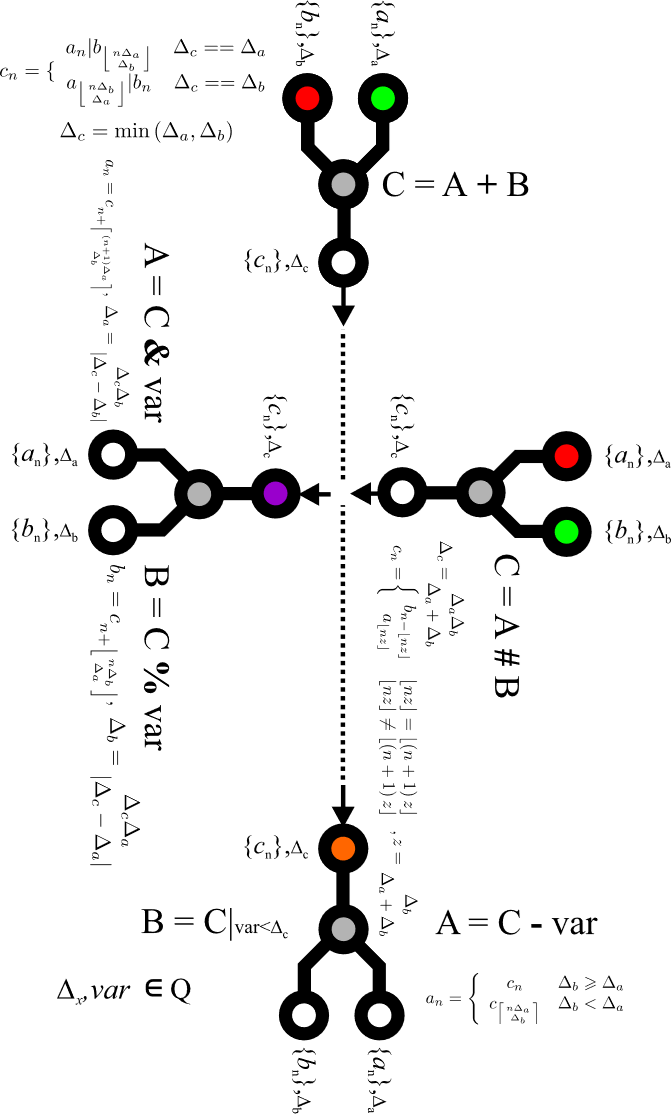
Fig. 2. Relationships between the algebra operators
Summary
I initially modeled these equations as Python programs. The formal form presented here took shape only at the very end of the search process. To numerically prove the correctness of the developed equations, I constructed sequences of operations on streams. If any elements got lost in the course of carrying out the operations shown, it meant I had made a mistake. It turns out, for instance, that it is essential in the implementation never to leave the domain of rational numbers, even for a moment. A mistake can be made by accident, by implicitly casting the result to a floating-point number. Materializing the result as a floating-point number must be deferred, in the calculations, until the result is explicitly carried over via the floor or ceiling operation. If we assemble a Python program into a sequence of operations on infinite streams and no data disappears as a result of that operation - we have an object ready for further research and formal analysis, ready for a formal mathematical proof of correctness. The formal proof (the mathematical formalism) can be found in the paper titled A Deterministic Method for Processing Data Sequences [3].
The branch of mathematics that contains the research related to these equations is called covering systems [4] within number theory.
ℹ️ Info
Presenting the mathematical foundations of the system is necessary in order to understand the further technical aspects of the solution. The methods presented go beyond the standard material currently taught in technical-science degree programs. This is because I drew the mathematical foundations from an area that, to my knowledge, had not previously been applied in engineering. These are methods that make it possible to build a new way of processing data. This is one of the aspects that sets RetractorDB apart from other similar solutions.
Query Language Construction
Communication between the developed system and the user takes place through a purpose-built, declarative query language. The language’s construction is based on the algebra presented in the previous chapter. Just as, for relational systems, relational algebra forms the basis for the SQL language - in our case, the developed algebra forms the basis for the RQL query language.
RQL stands for RetractorDB Query Language. Its syntax is very similar to SQL syntax. Bear in mind, however, that the correct term here is a False Friend. That is, it looks like SQL, but has little in common with it.
Valid statements in RQL currently begin with a handful of keywords. The most recognizable is the command starting with the keyword SELECT, followed by a list of attributes in the form of algebraic expressions - an algebra based on real numbers.
Statements are written in a text file. Its extension is conventionally .rql, but any other extension will also be accepted and processed. An RQL text file contains a sequence of statements beginning with defined keywords.
The # character starts a comment only when it is the first non-whitespace character on a line. The whole line, including an indented one, is discarded before parsing. Inside a FROM expression, # always means interleave regardless of whitespace. An end-of-line comment starts with //; block comments use /* ... */.
The query language was implemented using the Antlr4 parser generator [5]. The RQL grammar is written down, defined, and after every modification is compiled into the language in which RetractorDB itself was built. Every statement in a query file that is not a comment is compiled, processed, and modifies the system’s internal state. A statement may span multiple lines - line continuation is signaled with a \ character at the end of the line.
DECLARE Command
The DECLARE command is used to declare a data source.
Its syntax is described as follows:
DECLARE field type[N] [, field type[N]]
STREAM name, rate
BINFILE | TEXTFILE | DEVICE source
[TIMEOUT time]
[DISPOSABLE]
[ONESHOT]
[HOLD]
Fig. 3. DECLARE command syntax diagram
The railroad diagram in Fig. 3 was generated from the declare_statement rule in the system’s ANTLR4 grammar (RQL.g4). The diagram is read by following the lines from left to right: rounded green boxes are keywords and symbols entered literally, rectangles are values supplied by the user. A loop looping back through a comma means multiple field declarations are possible; the branch at the rate shows it can be written as a fraction (numerator/denominator) or as a single number; the branch before the source is the choice of the source kind (BINFILE, TEXTFILE, DEVICE or the deprecated FILE); the track bypassing TIMEOUT means the read deadline is optional, and its value - like the rate - is written as a fraction or a number; tracks bypassing DISPOSABLE, ONESHOT, and HOLD mean each of these directives is optional.
Source kinds
The data format follows from the keyword, never from the name or extension of the path:
| Keyword | What it reads | File kind at the path | After the end of data |
|---|---|---|---|
BINFILE | raw binary records whose size follows from the fields | regular file only | back to the beginning (loop), with ONESHOT end of source |
TEXTFILE | text: values separated by whitespace, the NULL token marks a missing value | regular file only | as BINFILE |
DEVICE | raw binary records from a live source; it interprets neither text nor the NULL token, a zero byte is zero | character device or FIFO | no writer: NULL records until data comes back; with ONESHOT end of source |
DECLARE MLII INTEGER, V1 INTEGER STREAM ecg, 1/360 BINFILE 'rec205'
DECLARE bp_coef INTEGER[25] STREAM bpf, 1 TEXTFILE 'bp_coef.txt'
DECLARE sample BYTE STREAM sensor, 0.02 DEVICE '/dev/urandom'
The extension selects nothing: BINFILE 'bytes.txt' reads raw bytes, and TEXTFILE 'values.dat' parses text.
DEVICE is a live source, so it takes neither DISPOSABLE nor HOLD - these directives apply to replayed files (BINFILE, TEXTFILE), see Read Options. It does take ONESHOT and its own TIMEOUT clause, described in Reading a DEVICE source and TIMEOUT. Opening a FIFO declared as DEVICE does not wait for a writer - the plan starts, and the writer may connect later.
The words BINFILE, TEXTFILE, DEVICE and TIMEOUT are reserved - no stream or field may be named that way (in lowercase either).
File kind check
Before the plan starts - also on a plan reload (xqry --reset) and on an ad hoc import (xqry -a) - the system checks the kind of file at the path of every declaration, without opening it. A path of the wrong kind (a directory, a block device, a socket, a FIFO for BINFILE/TEXTFILE, a regular file for DEVICE) refuses the plan with the stream name and the path, e.g.:
xretractor: stream 'src': BINFILE 'feed.fifo' is a FIFO, not a regular file
A path that does not exist is not a refusal: the stream then yields NULL records. Whether read warnings are available depends on the build mode, as described below for DEVICE. Compilation with -c does not perform this check - it does not have to run on the machine with the data.
Reading a DEVICE source and TIMEOUT
Reading a DEVICE source never waits without end and never holds up the rest of the system. The device or FIFO is opened and read without blocking, and the only waiting happens before the slot is computed, outside the data model locks. An xqry client therefore gets its answer also while the engine waits for device data, and the waiting time does not enter the measured slot computation time (E1).
The optional TIMEOUT clause gives the read deadline in seconds. The value is written the same way as the stream rate - as a fraction, a number with a point, or an integer:
DECLARE a BYTE STREAM s0, 1/50 DEVICE '/dev/sensor0'
DECLARE b BYTE STREAM s1, 1/50 DEVICE '/dev/sensor1' TIMEOUT 1/100
DECLARE c BYTE STREAM s2, 1/50 DEVICE '/dev/sensor2' TIMEOUT 0
| Value | Meaning |
|---|---|
TIMEOUT 0 | an immediate attempt: no complete record in a due slot gives a NULL record without waiting |
TIMEOUT t, t > 0 | one deadline for the whole record, counted from the start of the due slot; after it a NULL record |
| no clause | the deadline from the timeout_s key in the [sources] section of retractor.toml, and 0 without that key |
An explicit clause wins over the configuration - including an explicit TIMEOUT 0, which switches off a positive value from retractor.toml for a single source. A negative value is an error: there is no “wait forever” deadline. A deadline longer than a day is a plan error as well, and so is TIMEOUT on BINFILE, TEXTFILE and the deprecated FILE (on FILE with a hint to declare the source with an explicit DEVICE). The configuration key is described in Command-line options - xretractor.
Reading properties:
- The deadline is not renewed. A system call interrupted by a signal and a spurious wakeup do not extend the wait - the deadline is fixed from the start of the slot.
- Several sources wait in parallel. All
DEVICEsources due in a slot wait together, so the slot grows by at most the largest deadline, not by their sum. - An incomplete record survives the deadline. Bytes that arrived before the deadline wait in the source buffer; a record completed later goes to the next due slot. Only a record that is incomplete at the moment the writer disconnects is dropped - the record boundary is lost together with the writer, so the next writer starts a new record.
- The moment of reading. A
DEVICErecord consumed in slot k is read at the start of slot k, not at the end of the previous slot as forBINFILEandTEXTFILE. The logical record indices are the same: the same bytes given asBINFILEand through a FIFO asDEVICEgive the same results, also behind operators that join streams of different rates. - End of data. The end of data is decided only by a read returning zero bytes (a FIFO without a writer, a hung-up terminal). Without
ONESHOTit means “there is no writer right now”: the slot gets aNULLrecord, the source stays open, and a writer connecting again resumes the data. WithONESHOT(also in--until-eofmode) exhaustion is the first end of data after at least one byte was received - an end before the first data is a writer that has not connected yet. A writer that connects and disconnects without writing therefore does not end the run. - A read error other than a momentary lack of data (e.g. an unplugged USB device) gives
NULLrecords without exhausting the source. Reopening an unplugged device is not supported. - Mode without a clock. In
--no-clock(-f) mode the deadline of everyDEVICEsource is 0: real seconds have no conversion to virtual time. One immediate attempt in every due slot remains, so a FIFO with data written up front gives a repeatable run.
Dropped incomplete records and changes in the DEVICE connection state (no writer, resumed data, read error) have diagnostics at the WARN level. These warnings are available in the log in a Debug build; in Release, they are disabled at compile time by SPDLOG_ACTIVE_LEVEL=SPDLOG_LEVEL_ERROR. The absence of a warning in Release therefore does not confirm a successful read or complete records. Diagnostics at the ERROR level remain available.
The effective deadline of every DEVICE source and its origin (RQL, config, default or no-clock) goes to the engine log when the plan starts and on an ad hoc import, e.g. DEVICE stream 's1': effective TIMEOUT 0.01 s (RQL). The xretractor -c listing shows an explicit clause in the same form as the rate, e.g. timeout=1/100.
⚠️ Warning Limits of real time:
- Reading without blocking does not protect against a driver that blocks inside the read call despite the non-blocking mode. Such a device needs isolation in a separate process or thread.
- A deadline longer than the stream rate overruns the slot. Compilation then prints a warning, e.g.
DECLARE s1: TIMEOUT 0.05 s (RQL) is longer than the interval 0.02 s; waiting overruns the slot, taking the value fromretractor.tomlinto account as well.- Every clocked mode, with the
--realtimeoption and without it, schedules slots against a fixed anchor of the time axis. Waiting for aDEVICEsource that fits in the slot together with the computation does not shift the following slots. A longer wait delays the next slots, which are then made up without sleeping; if waiting and computation persistently exceed the period, the backlog grows - see Slot schedule.- The schedule does not synchronize the device clock. A producer persistently faster than the plan still builds a backlog in the source buffer. A persistently slower one lacks samples: this gives
NULLrecords in the ticks in which a record did not arrive in time, andTIMEOUTcan at most turn them into a delay growing together with the shortfall.
NOTE: Reading a
DEVICEsource,TIMEOUTand the end of data are covered by thedevice_timeouttest and by theut_faccbindevunit test.
Field types
Every field has a name and a type. Available types:
| Type | Size | Description |
|---|---|---|
BYTE | 1 B | unsigned 8-bit integer |
INTEGER | 4 B | signed 32-bit integer |
UINT | 4 B | unsigned 32-bit integer |
FLOAT | 4 B | 32-bit floating-point number |
DOUBLE | 8 B | 64-bit floating-point number |
STRING | N B | fixed-length byte string of length N |
Field arrays (type[N])
Any field can be given an array multiplier [N] - the field then occupies N × type_size bytes and creates N consecutive positions in the record schema:
DECLARE coef INTEGER[25] STREAM filter, 1 TEXTFILE 'coefficients.txt'
The field coef INTEGER[25] creates a record of size 25 × 4 = 100 bytes and gives access to indices filter[0] … filter[24]. This is the standard way of passing coefficient arrays (e.g. FIR filters) into the system.
Multiple fields of different types can be combined in a single record:
DECLARE id UINT, value FLOAT, name STRING[16] \
STREAM measurement, 0.1 \
BINFILE 'sensor.dat'
Record size: 4 + 4 + 16 = 24 bytes.
RetractorDB, running under Linux, reads and writes data to files. On Linux, access to most resources is carried out through access to various kinds of files. This approach unifies the way data is accessed.
An example of a command that creates an object in RetractorDB returning random values from the /dev/random stream 10 times per second, with values of type int, looks as follows:
DECLARE random_field INTEGER STREAM random_stream, 0.1 DEVICE '/dev/random'
A file declared as TEXTFILE is interpreted as a continuous, unbounded data file read line by line. Upon reaching the end of the file, reading resumes from the beginning. Basic support for the format is provided - if we specify two integer fields in the declaration, and the file contains two integer values separated by a space, those values will be read as consecutive elements of the record.
DECLARE field_1 INTEGER STREAM cyclic_stream, 0.1 TEXTFILE 'file.txt'
NOTE: The functionality described here is covered by the test:
Pattern7, described in the appendix Integration Tests.
A file declared as BINFILE is read as a sequence of raw records, also in a loop: after the last record has been read, the read position moves back to the beginning of the file.
The three optional directives (ONESHOT, DISPOSABLE, HOLD) control the lifecycle of file sources - a detailed description and comparison table can be found in the chapter Read Options.
Deprecated FILE form
DECLARE ... FILE 'path' is still accepted for backward compatibility. The source kind is then chosen by a fixed rule from the path - the same rule the system applied before the explicit keywords existed. The rows of the table are checked in order:
Path in FILE | Kind after translation |
|---|---|
contains .txt anywhere, regardless of case (data.txt, X.TXT, /x.txt.d/rec) | TEXTFILE |
starts with /dev/ | DEVICE |
| any other | BINFILE |
After translation the rules of the chosen kind apply, including the file kind check. A FILE pointing at a FIFO outside /dev is refused with a hint of the right keyword:
xretractor: stream 'src': BINFILE 'feed.fifo' is a FIFO, not a regular file (deprecated FILE resolved this path as BINFILE; declare it with DEVICE)
A FILE declaration resolved as DEVICE gets the whole DEVICE reading described above and takes ONESHOT, but not DISPOSABLE, HOLD or TIMEOUT - its deadline comes only from [sources] timeout_s or is 0. New plans should use the explicit keywords - the FILE form will be removed from the language in the future. FILE in the SELECT command still only names the result file and is not a deprecated form.
The warning about the deprecated form is silent by default, so existing plans do not change the program output. With --verbose (-v) xretractor prints one warning per declaration to stderr - at startup and in -c mode:
xretractor: warning: line 3: DECLARE core: FILE 'data.txt' is deprecated, resolved as TEXTFILE
On an ad hoc import (xqry -a) and on a plan reload (xqry --reset) the server’s --verbose decides, and the warning goes to the server’s stderr.
Source descriptor
The system writes the descriptor of every declaration in the storage directory as <stream_name>.desc: the fields, the path (REF) and the type (TYPE BINFILE, TYPE TEXTSOURCE or TYPE DEVICE). The descriptor stays between runs and on the next start it must match the plan also in type and path. Changing the source kind or the path while the descriptor is kept refuses the plan with the stream name:
xretractor: stream 'src': temp/src.desc was written for source 'v.txt' and the plan reads 'w.txt'; remove temp/src.desc to start the stream afresh
The exception is a descriptor written by earlier versions of the system for a regular binary file: it had TYPE DEVICE. If apart from the type it matches the plan, the start replaces it with a descriptor carrying TYPE BINFILE.
NOTE: Source kinds, the file kind check, the deprecated form and the descriptor are covered by the test
source_kinds.
ℹ️ Info
Support for NULL values (per field) is implemented in RetractorDB. Null metadata is stored in the
.metafile alongside the binary data, managed by themetaDataclass.
DECLARE Read Options
The DECLARE command accepts three optional directives that affect how a declared file source is read and its lifecycle:
DECLARE field type STREAM name, rate BINFILE | TEXTFILE source
    [DISPOSABLE]
    [ONESHOT]
    [HOLD]
The directives are independent and can be combined freely. They apply to replayed files (BINFILE, TEXTFILE). The live source DEVICE takes only ONESHOT of them, with the meaning described below - see the matrix at the end of the chapter. The read deadline of DEVICE is set by the separate TIMEOUT clause, described in the DECLARE Command chapter.
ONESHOT
Without ONESHOT, a file is read in an infinite loop - once the end of the file is reached, the read position returns to the beginning. ONESHOT disables the loop: the file is read exactly once, and once exhausted the stream returns records with every field marked NULL. The record bytes are zeroed, but the null markers distinguish missing data from a numeric zero. Exhausting the file neither ends the process nor deletes the file.
DECLARE measurement INTEGER STREAM burst, 0.1 BINFILE 'data.dat' ONESHOT
Use case: one-off loading of historical data into the system.
A DEVICE source has no file to rewind, so ONESHOT changes only the meaning of the end of data. Without ONESHOT the end of data means there is no writer: the slot gets a NULL record, and a writer connecting again resumes the data. With ONESHOT exhaustion is the first end of data after at least one byte was received; from then on the source returns only NULL records, also when another writer connects.
DECLARE sample INTEGER STREAM recording, 1/100 DEVICE '/tmp/recording.fifo' ONESHOT
The --until-eof (-u) option of xretractor reads all sources as if every declaration carried ONESHOT, and stops processing once the first of them is exhausted. For a DEVICE source exhaustion is checked before the slot that would get a NULL record from beyond the end of data, so such a record reaches no stream.
DISPOSABLE
When the source’s storage is closed - at the end of the process or when the plan is replaced - the system deletes the input file named in the declaration itself, the stream descriptor (.desc) and the metadata files (.meta, .meta.shadow), if they exist. The deletion depends neither on the end of the data nor on ONESHOT: a file read in a loop is deleted at closing as well, even if it was not read to the end.
DECLARE temp INTEGER STREAM one_time, 0.1 BINFILE 'temp.dat' DISPOSABLE ONESHOT
The combination DISPOSABLE ONESHOT is useful for temporary one-off input, but it is not required.
HOLD
The file is opened when the plan starts, but physical data reading is held until the first request for this stream’s data - fetching data by a query or preparing a record for a client (e.g. an Ad Hoc query). Merely listing the plan does not release the hold. Until the stream is queried, the system shows zero values for it; the first record of the file is read in the next step after the release. The hold is one-off - it does not return when the consumers go away.
DECLARE sparse INTEGER STREAM optional_stream, 1.0 BINFILE 'sparse.dat' HOLD
Use case: keeping the start of a recording until it is first needed, e.g. on user request via xqry. The combination ONESHOT HOLD replays the file once, from the moment of the first request.
Comparison table
| Directive | Read loop | Deletes files at closing | Delayed read start |
|---|---|---|---|
| (default) | yes | no | no |
ONESHOT | no | no | no |
DISPOSABLE | yes | yes | no |
HOLD | yes | no | yes |
Options and source kinds matrix
| Option | BINFILE | TEXTFILE | DEVICE |
|---|---|---|---|
ONESHOT | yes | yes | yes |
DISPOSABLE | yes | yes | no |
HOLD | yes | yes | no |
DEVICE with DISPOSABLE or HOLD is a compile error naming the stream and the option, e.g. DECLARE s: DEVICE does not take HOLD. The reasons: holding the reads does not stop the producer, it only builds up a backlog, and DISPOSABLE would delete the path of the device or FIFO, whose lifecycle does not belong to the reader. ONESHOT on DEVICE does not rewind a file, it only marks the end of data - see ONESHOT.
The deprecated FILE form resolved as DEVICE (a /dev/... path) behaves the same: it refuses DISPOSABLE and HOLD and accepts ONESHOT - see Deprecated FILE form.
SELECT Command
Every SELECT command in RetractorDB creates a continuous query. These queries run from the moment they appear in the system until the system shuts down.
The syntax of the SELECT command is as follows:
SELECT algebraic_expression [, algebraic_expression]
STREAM output_stream_name [instance_count]
FROM stream_algebraic_expression
[FILE 'artifact_file_name']
[RETENTION capacity [segments]]
[VOLATILE | PERSISTENT]
[STORAGE profile]
Fig. 4. SELECT command syntax diagram
The railroad diagram in Fig. 4 was generated from the select_statement rule in the system’s ANTLR4 grammar (RQL.g4). The diagram is read by following the lines from left to right: rounded green boxes are keywords and symbols entered literally, rectangles are values supplied by the user. The branch after the word SELECT shows that the field list is either an asterisk (the full record) or one or more expressions separated by commas (a loop looping back through a comma). An optional size in square brackets after the stream name creates a stream family. Tracks bypassing the FILE, RETENTION (with an optional second parameter - the number of segments), VOLATILE/PERSISTENT, and STORAGE clauses mean each of them is optional.
Readers familiar with SQL will immediately notice that the command shown above differs significantly from what they know from relational databases.
The first difference, beyond syntax, is that once entered into the system, these commands run until the system shuts down. Every SELECT command is a continuous query. The STREAM clause requires the author to give every query a unique name. While the algebraic expressions in the SELECT clause’s field list don’t differ from the form familiar from relational systems, the stream algebraic expression must satisfy the conditions presented in the previous chapter on algebraic expressions. The optional FILE and RETENTION clauses provide processes for directing results and managing their retention. Old, segmented output files can be deleted on an ongoing basis, keeping room in the system for new data in continuous motion.
An example of a query creating a new data stream might be the following RQL command.
SELECT str1[0]*10 + str1[1]*10, str1[2] STREAM str1 FROM A+B
A query built this way assumes that someone has declared streams A and B. This could have been done with the DECLARE keyword or with another SELECT command. Based solely on the line containing the query, we cannot tell how fast the data of stream str1 arrives. This information is computed at compile time, based on streams A and B and the algebraic expression in the FROM clause.
Stream generators
An optional size after the name in the STREAM clause expands one template into that many queries. The $ symbol denotes a zero-based instance ordinal:
DECLARE cell INTEGER[4] STREAM cells, 1/10 TEXTFILE 'cells.txt'

SELECT cells[$] STREAM cell[4] FROM cells
SELECT *        STREAM grouped FROM cell[0]#cell[1]#cell[2]#cell[3]
The first SELECT creates the physical streams cell$0, cell$1, cell$2, and cell$3. A reference such as cell[2] in the FROM clause denotes instance cell$2; in a SELECT-list expression, cells[2] still denotes field index 2.
Within a template, $ may occur:
- as a field index, for example
cells[$]orcells[3-$]; - as an expression value, for example
cells[0]+$; - in a reference to another family in the
FROMclause, for examplecell[$]@(2,4).
A generator-index expression is integral and may contain literals, $, parentheses, and the operators *, +, and -. The family size must be positive and the template must actually use $. A generator cannot carry a FILE clause because one file name cannot serve multiple streams. The compiler also rejects family indices outside the declared range, negative field indices, field indices beyond the source’s slots, and collisions between generated and existing stream names. The field-index range is checked by the same rule as for a hand-written index - see Index out of range.
Expansion is the compiler’s first pass. Afterwards the plan is identical to one containing hand-written cell$0…cell$3 streams; runtime has no separate generator mechanism.
A generator may cover successive stages of the same pipeline. This lets one computation be written once and applied independently to every input channel:
DECLARE sample INTEGER[8] STREAM samples, 1/1000 TEXTFILE 'samples.txt'

SELECT sample[$]^2 STREAM square[8] FROM samples
SELECT *           STREAM energy[8] FROM SUMC(square[$]@(25,100))
This creates eight pairs of square$N and energy$N streams, one per channel. The $ symbol selects a family-instance ordinal while the template is expanded. Do not confuse it with [_], which replicates a field expression within one query according to the flattened input schema.
NOTE: Generator syntax, including
[$], is checked by thestream_generatorintegration test and byut_compilercases intest/UnitTest/test_compiler.cpp. Record-window aggregates are checked bywindow_aggregate. Integration tests are described in Integration Tests.
The VOLATILE clause creates an ephemeral form of the query. Its data remains in an in-memory buffer whose capacity the compiler sets to meet the plan’s needs; only the descriptor describing the data structure appears on disk.
The STORAGE clause allows choosing how the artifacts created are managed and stored. The full table of types, with a description of each, is in the chapter Storage Types.
FROM clause operators
The stream algebraic expression in the FROM clause can include:
| Operator | Syntax | Description |
|---|---|---|
| Sum | A + B | Concatenates the schemas of two streams - see Summation Sequencing |
| Interleave | A # B | Interleaves two streams - see Interleaving Sequencing |
| Shift | A > N | Shifts reads by N samples |
| Interval conversion | A - r | Retimes a stream to rational interval r |
| De-interleave | A & r / A % r | Recovers the left or right interleave component for ratio r |
| AGSE window | A @ (k, w) | Builds a sliding data window - see AGSE Sliding Data Window |
| Reduction | MIN(A) / MAX(A) / AVG(A) / SUMC(A) | Reduces a multi-field record to one value - see Aggregate Operators |
MIN/MAX/AVG/SUMC(expression : W) aggregates occur in the SELECT list rather than the FROM stream expression. They reduce W historical records and may be operands in a larger field expression, for example 2*MIN(a : 5)+1. See Aggregate Operators for both aggregation axes.
Precedence and associativity
From strongest to weakest binding:
- a reducer call, stream name, or parenthesized expression;
- the chainable postfix operators
@,&,%,>,-, and the deprecated.aggregatorform; - interleave
#; - sum
+.
The binary operators # and + are left-associative. Postfix operators also compose from the left, so A@(1,4)&2 means (A@(1,4))&2.
⚠️ Warning
A#B>NmeansA#(B>N), because shift binds more tightly than interleave. To shift the interleave result, write(A#B)>N. The same rule applies toA#B-r.
Whitespace around # does not affect its meaning: A # B and A#B are the same interleave.
Field expressions
The SELECT list and RULE conditions use scalar expressions containing field references, arithmetic operators, NULL values, and functions. The complete syntax, precedence, function list, and conversion rules are documented in Field Expressions and Scalar Functions.
Exponentiation
The ^ operator exponentiates numeric values in the SELECT list and in RULE conditions. It binds more tightly than * and /, which in turn bind more tightly than + and -. Exponentiation is right-associative:
SELECT v*w^2, v^w^2 STREAM powers FROM source
This means v*(w^2) and v^(w^2). Writing (v*w)^2 requires explicit parentheses.
For integer and rational types, a non-negative integral power has exactly the semantics of repeated multiplication, including type promotion and overflow. Other cases use floating-point computation; an infinite or NaN result becomes NULL. Text operands are not allowed.
ℹ️ Info A negative literal is one grammar atom:
-2^2means(-2)^2. For a field,-v^2means-(v^2). Use parentheses whenever the intended grouping might be unclear.
⚠️ Warning After an interleave
A#B, do not refer to its components asA[0],A.field,A[_], orA.*. An interleave has one shared schema; use the output stream name or recover a component with&/%. See Aliasing for details.
NOTE: The shift operator
A > Nis covered by the test:issue56_timeshift, described in the appendix Integration Tests.
NOTE: Null-value propagation through SELECT expressions is covered by the test:
issue121_null_propagation, described in the appendix Integration Tests.
DEFAULT VOLATILE sets default volatility for the plan. PERSISTENT overrides it for one result. See VOLATILE and PERSISTENT.
Field Expressions and Scalar Functions
A field expression computes one value of an output record. It occurs in the SELECT list, in a RULE condition, and as the argument of a record-history aggregate. Do not confuse it with the stream expression in FROM, which constructs and schedules an entire stream.
Building an expression
Operands are numeric and text literals, $ inside a stream generator, field references, and function results. A field may be addressed by name, stream-qualified name, or flat index, for example temperature, src.temperature, and src[0]. For a numeric declaration a T[N], bare a denotes the complete array entry and is not a scalar operand; use a[0]…a[N-1]. STRING[N] is one text field.
The basic arithmetic operators are +, -, *, /, and ^. Parentheses change grouping. * and / bind more strongly than + and -; exponentiation ^ binds most strongly and is right-associative:
SELECT v*w^2, v^w^2, (v*w)^2 STREAM powers FROM source
These fields mean v*(w^2), v^(w^2), and (v*w)^2. A negative literal is one grammar atom: -2^2 means (-2)^2, while -v^2 means -(v^2).
For integer and rational types, a non-negative integral power has the semantics of repeated multiplication, including type promotion and overflow. Other cases use floating-point computation; an infinite or NaN result becomes NULL. Text operands are not allowed.
NULL propagates through ordinary arithmetic. Division by zero yields NULL for every numeric type and does not stop later stream processing. Comparison and three-valued logic in a RULE condition are documented in Logical Condition.
Addition, subtraction, and multiplication on UINT fields are checked: a sum or product outside the unsigned 32-bit range, or a negative difference, yields NULL instead of a wrapped value. An operation on an INTEGER and a UINT operand is computed on the exact values, and only the result is narrowed to UINT: it yields NULL only when the result does not fit. With u = 10 and i = -2, u + i yields 8 while u * i yields NULL; comparing such a pair, for example i < u, is exact as well. INTEGER and RATIONAL arithmetic also yields NULL on overflow.
⚠️ Warning After an interleave
A#B, do not refer to its components asA[0],A.field,A[_], orA.*. An interleave has one shared schema; use the output stream name or recover a component with&or%. See Aliasing.
Unary operators
The behavior in this section requires an engine version containing the fix for #328.
The operators +, -, and ~ accept a field, a function result, or a parenthesized expression. Each item in the SELECT list still produces one output field, and an operand in a RULE condition remains part of that condition.
| Operator | Operand type | Result |
|---|---|---|
+a | Any value type, including STRING | The value and type of a, unchanged |
-a | INTEGER, RATIONAL, FLOAT, DOUBLE | Arithmetic negation, preserving the type |
-a | BYTE, UINT | Bitwise complement, preserving the type; the same result as ~a |
~a | BYTE, UINT | Inversion of all bits within the operand type’s width |
For a BYTE value of 0, both -a and ~a yield 255; for 1 they yield 254, and for 255 they yield 0. For UINT, the corresponding results for 0 and 1 are 4294967295 and 4294967294. This is neither subtraction from zero nor logical NOT. To obtain an arithmetic negative value from an unsigned field, explicitly convert its type first, for example -to_double(a).
The type is that of the computed operand, rather than just the source field. The literal -1 is a negative INTEGER; it does not use the bitwise-complement rule for BYTE or UINT. An allowed operator passes NULL through unchanged. Overflow in arithmetic negation of an INTEGER or RATIONAL yields NULL; for example, -a over an INTEGER value of -2147483648 yields NULL.
The operand of a unary operator includes exponentiation, multiplication, and division, but stops before binary + or -. Thus -a+1 means (-a)+1, while -(a+1) negates the entire sum. -a*b means -(a*b); write (-a)*b to negate only a. This distinction can change the operand type, the bitwise-complement result, or where overflow occurs. Likewise, ~a*b means ~(a*b). The exponentiation distinction remains: -2^2 yields 4, whereas -a^2 means -(a^2); write (-a)^2 to square a negated field.
DECLARE b BYTE, u UINT, i INTEGER STREAM src, 1 TEXTFILE 'source.txt'
SELECT -src[0], ~src[0], -src[1], ~src[1], +src[2], -(src[2]+1), -src[2]+1 STREAM unary FROM src
RULE negative ON unary WHEN -unary[4] < 0 DO DUMP -1 TO 0
For input 0 1 5, the result has seven fields: 255, 255, 4294967294, 4294967294, 5, -6, -4. The rule checks the negation of the fifth field, that is -5 < 0.
-a over STRING and ~a over INTEGER, RATIONAL, FLOAT, DOUBLE, or STRING are rejected during compilation, both in SELECT and in a RULE condition. Diagnostics state the reason: unary '-' is not defined for STRING or unary '~' is defined only for BYTE and UINT, not for .... When checking a file with xretractor -c, the reason appears in Check result:. Rejecting such an ad-hoc query (xqry -a) leaves the running plan and service active.
Available scalar functions
The sole name-and-arity list shared by the compiler and evaluator is the rqlFunctions.hpp table. Matching is case-insensitive and the canonical spelling is stored in the plan. An unknown function or invalid arity stops compilation rather than being deferred to runtime.
| Group | Functions |
|---|---|
| Mathematical | Sqrt, Ceil, Floor, Abs, round, trunc, sin, cos, exp, tan, log, log2 |
| Value handling | isnull, null2zero, IsZero, IsNonZero, Length |
| Conversions | to_integer, to_float, to_double, to_string |
Every function takes one expression argument. The only exception is the optional output field width in to_string(expression : width).
Predicates and missing values
isnull(x)returns 1 for NULL and 0 for a present value;null2zero(x)maps NULL to integer zero but passes a present value without changing its type;IsZero(x)andIsNonZero(x)return integer 1 or 0 for a numeric argument.
null2zero is lossy: afterwards, an original missing value cannot be distinguished from an actual zero. It does not replace the NULL bitmap stored in .meta.
String length
Length(x) accepts a string only. It counts the actual value up to the first zero byte, not the declared STRING[N] width. A STRING[8] field containing alpha therefore yields 5. A numeric argument is a runtime error.
Conversions
to_integer, to_float, and to_double convert a numeric or textual value to the named type. NULL passes through unchanged. to_integer truncates toward zero rather than flooring: to_integer(-8/3) yields -2. A floating-point value that INTEGER cannot hold - NaN and infinity included - yields NULL, exactly like arithmetic overflow. The same rule covers mathematical functions over an integer field whose result returns to the argument type: Sqrt(-4) and log(0) over an INTEGER field yield NULL. The range is checked after truncating the fractional part: for a DOUBLE argument, the value 2147483647.5 yields 2147483647, whereas 2147483648.0 yields NULL. The rule does not stop at integer types: NaN and infinity have no rational approximation, so a floating-point value written into a RATIONAL field yields NULL just as it does for INTEGER, not zero.
Converting an integer or rational value to a narrower integer type also yields NULL if the result does not fit: this includes a negative value directed to UINT, a UINT above INT_MAX directed to INTEGER or RATIONAL, and a value outside 0..255 directed to BYTE. Conversion from RATIONAL to an integer type first truncates toward zero, then checks the range. Invalid numeric text yields NULL. Approximation of a finite floating-point number as RATIONAL stops at the last fraction whose numerator and denominator both fit in int. For a finite FLOAT or DOUBLE argument, the integer part of its absolute value is checked first: 2147483647.5 and -2147483647.5 can be approximated, while 2147483648.0 and -2147483648.0 yield NULL.
to_string creates a text field. Without a second part its width is 32 bytes; to_string(x : N) declares N bytes. The separator is a colon because a comma separates fields in the SELECT list:
N must be in 1..65536. to_string(x : 0) is a parser error (to_string width 0 must be greater than zero), and the resulting string concatenation must also fit the field limit. See Plan Size Limits.
SELECT to_string(value : 10), Length(label), null2zero(optional) \
STREAM converted FROM source
The output text width is inferred after field references have been resolved, so a pure copy of STRING[N] and text concatenation retain the correct descriptor. The type of the whole expression, including numeric expressions, is determined by compiler::inferFieldShapes() after field references are resolved; see Type Promotion.
The declared width is a property of the field, not a side effect of one particular compilation pass. It also holds when the whole argument is constant: to_string(42 : 16) yields STRING[16], not STRING[2]. Expression simplification folds the argument underneath the call but never removes to_string itself - otherwise the declaration would disappear together with the program on a second compilation of the plan, that is after an ad-hoc query (xqry -a), which compiles the live plan a second time.
sin, cos, and exp
All three functions take a numeric argument and return DOUBLE, regardless of the argument’s type. sin and cos interpret angles in radians. For an INTEGER field k, the expressions sin(k), cos(k), and exp(k) therefore produce DOUBLE fields without truncating fractional results. A NULL argument yields NULL; a non-finite result, such as exp(1000), also yields NULL without stopping the stream.
A RATIONAL argument is the exception: the compiler rejects it and requires an explicit to_double, exactly as it does for Sqrt - see the section below.
Changing the result type of sin and cos can change the .desc descriptor and record layout relative to an older engine: INTEGER and FLOAT occupy 4 bytes, while DOUBLE occupies 8. An existing artifact with the old schema must be recreated or written to a separate output stream.
Irrational functions over a RATIONAL value
Sqrt, sin, cos, exp, tan, log, and log2 do not accept a RATIONAL argument - the compiler rejects such a query through the Check result: channel and names the workaround. In practice this concerns stream reducers over BYTE, INTEGER, UINT, and RATIONAL fields, whose result type is RATIONAL. Reducers over FLOAT and DOUBLE preserve the input type:
SELECT * STREAM m FROM AVG(src)
SELECT Sqrt(m[0]) STREAM o FROM m              // rejected at compilation
SELECT Sqrt(to_double(m[0])) STREAM o FROM m   // correct
One rule applies: a function with an irrational range over an exact rational value requires an explicit to_double. The same rule covers a rule condition (RULE ... WHEN), which the compiler checks in a separate pass.
For Sqrt, tan, log, and log2, the reason for the gate is the return from a double calculation to RATIONAL: the result used to be approximated by a fraction with a large denominator (for the rational argument 2/1, the square root yielded 19601/13860 and the logarithm 2731/3940). In an older version, two further multiplications of such an approximation could silently overflow its 32-bit numerator or denominator; Sqrt(x)*Sqrt(x)*Sqrt(x) returned -4.247 instead of +2.828. Arithmetic on INTEGER and RATIONAL field values now detects overflow and writes NULL, but these functions still require an explicit to_double.
For sin, cos, and exp the reason is different: these three end at DOUBLE and never return to RATIONAL, so they would compute correctly. Their rejection is a language contract decision, made so that no list of exceptions has to be remembered - one rule instead of seven separate behaviours. The price is a to_double in every query computing, say, an RMS over a reducer.
The restriction extends neither to the remaining functions nor to other argument types. The rounding functions Floor, Ceil, round, and trunc over RATIONAL are safe, because their result is integral and therefore has denominator 1, and Abs operates on the value directly and never touches the denominator.
The gate covers only the pairing with RATIONAL and changes no function’s result type. tan, log, and log2 over INTEGER still yield INTEGER, that is, they truncate the fractional part - an explicit and intended loss, not an overflow. Bringing them to DOUBLE, as sin, cos, and exp are, would change the field type in .desc, so it is a separate task.
NOTE: Functions and type propagation are covered by the integration tests
fncall_runtime_case,string_field_passthrough,issue121_isnull,issue128_numeric_to_string, andissue128_string_to_numeric, and by theut_compiler,ut_expeval, andut_facctxtsrcunit tests.
Summation Operation Sequencing
Data flows into the system and is processed within it. The order in which it arrives and is processed can be described by the term sequencing. The way data is combined is described by the algebraic expression placed in the FROM clause. These expressions are written as a series of algebraic operations subject to strict rules - rules similar to those we learned in elementary school, governing arithmetic operations on numbers such as addition, multiplication, division, and subtraction.
Let’s start by analyzing the following query:
DECLARE a BYTE STREAM A, 1 TEXTFILE 'data1.txt'
DECLARE a BYTE STREAM B, 2 TEXTFILE 'data2.txt'
SELECT * STREAM str1 FROM A+B
I’ll save the query in a file named qplan1.rql. Then I’ll run the following commands:
$ xretractor -c qplan1.rql -w 1:3 > out.txt
$ swirly out.txt -o out.svg
The swirly program was installed from its GitHub repository [6]. This program is used to generate marble diagrams used to explain the behavior of RxJs asynchronous operations [7].
The modification I applied for my use case is an alternative meaning for the vertical lines. In my case, vertical lines separate uniform time intervals - showing the number of cycles requested at invocation time (in this case, 3 cycles). The generated image is shown in Fig. 5:
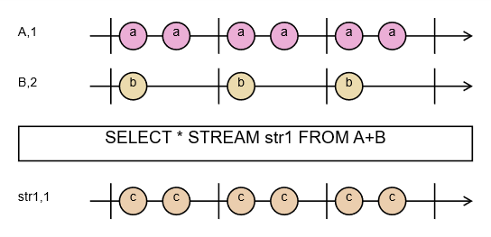
Fig. 5. Marble diagram - the sum operation
A few words of explanation are needed here about this generator and how its input is produced. I built into the compiler an option for visualizing the execution of a sequence of operations. Diagrams produced by the Swirly program are one convenient way of presenting time dependencies. On input, the Swirly program expects a text file describing the diagram. A generator that simulates the requested number of cycles and builds a file for Swirly has been built into the compiler.
When xretractor is given, as its first parameter, the name of the file containing the query execution plan, it requires a second parameter ( -w [–diagram] ) - indicating that we expect marble-diagram output. The required argument of the -w parameter is two numbers separated by a colon. The first tells the program whether to insert time separators into the diagram (the vertical lines separating cycles); the second parameter is how many cycles should be shown in the diagram.
If you look at the generated out.txt file, you’ll see the following content:
% Creating diagram output grid is on, cycle count:3
% Minimum interval is 1000ms
% Maximum interval is 2000ms
% Grid time is 500ms, divider:2
% Full cycle step count in grid is 4
-|a-a-|a-a-|a-a-|-
title = A,1

-|b---|b---|b---|-
title = B,2

> SELECT * STREAM str1 FROM A+B

-|c-c-|c-c-|c-c-|-
title = str1,1
In this file, note the data shown in the comments. These are the times computed while generating the diagram, relative to the scale shown in the marble diagram. As you can see, for our query the minimum window interval is 1 second and the maximum is 2 seconds. The identified and computed grid is half a second. On the diagram, each letter or dash represents a half-second period between successive operations.
We can manually change the generated content. If we replace the content as follows:
-|a-b-|c-d-|e-f-|-
title = A,1

-|g---|h---|i---|-
title = B,2

> SELECT * STREAM str1 FROM A+B

-|j-k-|l-m-|n-o-|-
title = str1,1
j:=ag
k:=bg
l:=ch
m:=dh
n:=ei
o:=fi
and then run the swirly program again, we’ll see a more detailed picture showing the sequence of events occurring in the system.
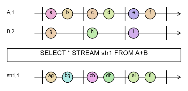
Fig. 6. Marble diagram - Sum, modified diagram
In the diagram shown in Fig. 6, you can see which marbles were joined and which marbles they were formed from. Remember, though, that this is a manually corrected image, made for the purposes of this work - the generator built into the compiler does not implement this functionality.
NOTE: The functionality described here is covered by the tests:
Pattern1,issue167_triarg, described in the appendix Integration Tests.
The same name more than once in FROM
A stream may appear in a FROM expression more than once - directly and under another operator, e.g. bar + MAX(bar) or src + src>1, or twice under different operators, e.g. src@(1,5) + src@(2,3). The input record then holds a separate block of fields for each occurrence, and a reference by name (bar[0], src[4]) as well as the SELECT * expansion must point to one of them. The compiler picks the first occurrence in a fixed order: first the direct operands of the expression in the order they are written, only then the streams nested under operators (a reducer, a shift, a window), also in the order they are written. The index range check uses the same order, so the bound of src[k] is measured on the occurrence the reference will actually read.
DECLARE v INTEGER[3] STREAM bar, 1/50 TEXTFILE 'a.txt'
SELECT * STREAM chk FROM bar + MAX(bar)
The chk stream has four fields: the three fields of the bar that stands directly in FROM, and the record maximum. A direct operand always points to its own fields, even when it is written second: in src>1 + src the reference src[0] reads the current sample, not the shifted one. In src@(1,5) + src@(2,3) the name src is reachable only through windows, so it points to the first of them: src[4] is valid, and src[5] is a compilation error. To refer to the fields of the second occurrence, give it its own name in a separate query, e.g. SELECT * STREAM w2 FROM src@(2,3), and use w2 in the FROM expression.
NOTE: The first-occurrence rule is checked by the
ut_compilerunit tests:direct_operand_keeps_its_own_slots_beside_a_nested_occurrenceandrange_check_and_offset_agree_on_a_name_reached_twice.
Interleaving Operation Sequencing
Let’s now analyze the interleaving operation. Let’s create a file qplan2.rql with the following content:
DECLARE a BYTE STREAM A, 1 TEXTFILE 'data1.txt'
DECLARE a BYTE STREAM B, 2 TEXTFILE 'data2.txt'
SELECT * STREAM str1 FROM A#B
Aside from the # symbol instead of the + symbol in the from clause, the two files are identical. Let’s run the compilation and the swirly program. The resulting graphic will look as follows:
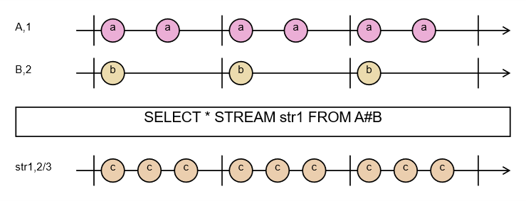
Fig. 7. Marble diagram - the interleaving operation
In Fig. 7 we see a change. The marbles of stream str1 have been evenly arranged in time. The events occurring in the declared input data streams have not changed. What has changed is the way the output stream str1 is built.
If we look at the generated text schema, we’ll see that the time values have changed too:
% Minimum interval is 666ms
% Maximum interval is 2000ms
% Grid time is 333ms, divider:2
% Full cycle step count in grid is 6
I encourage further experimentation with this way of presenting the defined operations on time series.
NOTE: The functionality described here is covered by the tests:
operations,Pattern1, described in the appendix Integration Tests.
VOLATILE Clause
The VOLATILE clause in the SELECT command creates a stream stored in memory. On disk, only the .desc descriptor file describing the data schema appears - the data itself is never written.
Default volatility and the PERSISTENT exception
DEFAULT VOLATILE selects in-memory storage for SELECT results without an explicit policy and for compiler-generated substrates. It replaces repeated VOLATILE clauses and the SUBSTRAT 'memory' directive:
DEFAULT VOLATILE
DECLARE a INTEGER STREAM sensor, 0.1 DEVICE '/dev/sensor0'
SELECT sensor[0]*100 STREAM scaled  FROM sensor
SELECT scaled[0]     STREAM history FROM scaled PERSISTENT
scaled stays in memory, while history writes data to disk using the usual FILE, RETENTION, and STORAGE settings. PERSISTENT affects only that SELECT result; its substrates still inherit the default volatility.
The directive may appear once, before the first DECLARE, SELECT, or RULE. It does not change DECLARE sources. Programs without it retain their existing settings. VOLATILE and PERSISTENT are mutually exclusive clauses.
An explicit STORAGE profile on a SELECT overrides the default; for example, STORAGE DEFAULT selects ordinary file storage. Explicit VOLATILE retains its precedence over STORAGE. Combining PERSISTENT STORAGE MEMORY is an error. Explicit SUBSTRAT 'profile' selects substrate storage regardless of the order of the two directives in the header. FILE or RETENTION alone does not disable default volatility: add PERSISTENT to store history. RETENTION capacity segments on an in-memory stream is a compilation error with that hint.
Behavior
SELECT expression STREAM name FROM source VOLATILE
The parser initially sets the storage type to MEMORY with a capacity of 1, or n from a RETENTION n clause:
if (ctx->VOLATILE() != nullptr || inheritVolatile) {
    qry.policy = std::make_pair("MEMORY", std::max<size_t>(qry.policy.second, 1));
}
The compiler then determines the capacity required by the plan. If another stream reads the history of a VOLATILE result, the buffer may hold more than one record. This means that:
- the in-memory buffer holds at least the most recent record and any history its consumers need,
- data never reaches disk,
- the
.descdescriptor is still created - other processes can learn the stream’s schema.
The ring has capacity max(RETENTION n, plan need, 1) and counts against [limits] history_memory_mib. Attaching an ad-hoc DO DUMP -H TO M rule requires H+1 slots, including the current record. For H > 0, the server rejects the request when capacity N <= H; the ring cannot be enlarged in a running plan. See Alerting implementation for the rules on waiting for history. See Plan Size Limits.
Difference from STORAGE MEMORY
| Property | VOLATILE | STORAGE MEMORY |
|---|---|---|
| Buffer capacity | 1 record or RETENTION n; may grow to meet plan needs | 1 record or RETENTION n; may grow to meet plan needs |
RETENTION n clause | ring size | ring size |
RETENTION n s clause | compilation error | compilation error |
Precedence over STORAGE | yes | - |
| Descriptor on disk | yes | yes |
| Data on disk | no | no |
VOLATILE is useful when the query result is being pulled by xqry on an ongoing basis and history is not needed - e.g. the current value of a sensor exposed by the operating system.
Example
DECLARE a INTEGER STREAM sensor, 0.1 DEVICE '/dev/sensor0'

SELECT sensor[0] * 100 STREAM scaled FROM sensor VOLATILE
The scaled stream contains, at every moment, a single, current value. The xqry process can read it via shared memory.
STORAGE Types
The STORAGE clause in the SELECT command, and the SUBSTRAT directive, accept one of the following identifiers. Each maps to a specific data-accessor class in the implementation.
Type table
| Keyword | C++ class | Retention | Shadow | Purpose |
|---|---|---|---|---|
DEFAULT | groupFile<posixBinaryFileWithShadow> | yes | yes | Default production mode; a .shadow file protects modifications |
DIRECT | groupFile<posixBinaryFile> | yes | no | Retention without shadow protection |
MEMORY | memoryFile | yes (RAM) | no | Data in memory only; circular buffer, never written to disk |
POSIX | posixBinaryFile | no | no | A single binary file; no retention |
POSIXSHD | posixBinaryFileWithShadow | no | yes | A single file with shadow protection; no retention |
GENERIC | genericBinaryFile | no | no | Generic binary file |
Any other value in STORAGE or SUBSTRAT is a compile error. The DECLARE source types - BINFILE, TEXTSOURCE and DEVICE, written to the TYPE field of the source descriptor - are not storage profiles: their accessors (binaryDeviceRO, textSourceRO) are read-only, so a SELECT result cannot be created in them. The source kind is chosen by the keyword in DECLARE.
The refusal names the stream and the allowed profiles:
STORAGE DEVICE of stream dst is not a storage profile but a source kind of DECLARE; use DEFAULT, MEMORY, DIRECT, POSIX, POSIXSHD or GENERIC
In the STORAGE clause a profile, like every keyword, has two spellings - upper case or lower case (MEMORY, memory); Memory is an error. The value of the SUBSTRAT directive is a string and its case does not matter.
Retention - artifacts are rotated, older files are deleted automatically (requires RETENTION capacity segments on SELECT).
Shadow - every modification is written to a separate .shadow file; historical data is protected from being overwritten.
For MEMORY, retention works in memory as a circular buffer: successive appends overwrite the oldest slot (index % capacity). Data is not segmented into files and never reaches disk. RETENTION n sets the ring size (at least what the plan needs) - the same for STORAGE MEMORY and VOLATILE; the segmented form RETENTION n s is a compilation error here.
Even without RETENTION, a MEMORY store has a finite capacity: at least one record, increased by the compiler to meet consumer needs. Formerly, STORAGE MEMORY could grow without bound or, with RETENTION n, write to disk under the wrong storage type. The ring size and total history cost now count against the plan budget. An ad-hoc DO DUMP -H TO M rule requires H+1 slots for history plus the current record. For H > 0 and capacity N <= H, the request is rejected; attaching a rule does not enlarge a live store. See Alerting implementation for the rules on waiting for history.
Retention on disk
The DEFAULT and DIRECT stores keep data in segments: RETENTION capacity segments keeps at most segments files of capacity records each, and the oldest segment is deleted when a new one is opened. The one-argument form RETENTION n means only the size of a MEMORY ring; on a file store it is a compilation error with the hint RETENTION n <segments>. segments = 0 means “no segment limit”.
For example, RETENTION 100 STORAGE DIRECT is rejected because it omits the segment count. Write RETENTION 100 4 STORAGE DIRECT instead. For STORAGE MEMORY the rule is reversed: RETENTION 100 sizes the ring, while RETENTION 100 4 is rejected as segmented retention on a RAM store.
Right after a rotation only (segments - 1) * capacity + 1 records remain on disk. A plan that reads further back into the stream (a >N shift, an @ window, a DUMP range) is a compilation error - reading a deleted segment would stop the running server.
A file stream without RETENTION, with segments = 0, or in a store without retention (POSIX, POSIXSHD, GENERIC) grows on disk without bound. This is allowed - durable history. With --verbose, xretractor lists such streams on stderr, both at startup and in -c mode, including with --quiet and for intermediate streams extracted by the compiler. Without --verbose, this list does not appear on stderr; WARN diagnostics in the log depend on the logging configuration and are disabled in Release builds. The operator can bound every DEFAULT/DIRECT stream without RETENTION with the key default_retention = [capacity, segments] in the [storage] section of retractor.toml. Without that key, history limits come from explicit RETENTION; startup cleanup is described below.
A start without the ROTATION directive begins SELECT outputs and substrates from scratch: it deletes their whole file families - data with its .shadow file, .desc, .meta, and retention segments. It does not delete DECLARE source files. With ROTATION, retained disk-store files must match the plan: if a kept .desc has another storage type or retention, the start (and xqry --reset) is refused, naming the stream and both configurations. For MEMORY, old descriptor and metadata files are removed even under ROTATION, so the new ring cannot inherit the previous plan’s configuration. Changing the capacity over kept segments would shift record addressing, so the operator chooses: restore the previous configuration in the plan, or remove the stream’s files.
NOTE: The
MEMORYtype (SUBSTRAT ‘memory’) is covered by the tests:issue61_tmpmem(serial and parallel), described in the appendix Integration Tests.
Links in storage paths
Storage writes refuse to follow a symbolic link at the final data, shadow, metadata, or descriptor filename. An explicit caller-supplied REF can authorize a main data-file link; the exception covers neither retention-segment names nor auxiliary files. Links in parent directories remain permitted. See Files for refusal behavior, the REF exception, and the protection boundary.
When to use which
The choice depends on the environment’s requirements:
- Production environment, critical data →
DEFAULT(retention + shadow) - Production environment, historically insignificant data →
MEMORY(zero disk usage, retention in RAM) - Development and debugging →
DEFAULTorDIRECT(data visible on disk) - Reading from a binary file, a text file or a device → not through
STORAGE, but through the source kind inDECLARE(BINFILE,TEXTFILE,DEVICE)
Example
SELECT str1[0] STREAM str1 FROM core0 STORAGE MEMORY
SELECT str2[0] STREAM str2 FROM core0 RETENTION 100 4 STORAGE DIRECT
For substrates globally - the SUBSTRAT directive:
SUBSTRAT 'memory'
Aggregate Operators
Two aggregation axes (MIN, MAX, AVG, SUMC)
The same four keywords describe two different constructs. In FROM, a reducer folds the fields of one current record. In the SELECT list, a record-history aggregate folds one expression value evaluated for each consecutive historical record. The location therefore determines whether reduction runs horizontally across fields or vertically across time.
Current-record reducers in FROM
Stream reducers operate on a stream with multiple fields - typically the output of the @(k,w) operator or a record that contains a numeric array. They reduce all flat slots of one record to one value.
Syntax
FROM AGGREGATOR(stream_expression)
where AGGREGATOR is one of:
| Keyword | Behavior |
|---|---|
min / MIN | minimum of all fields in the record |
max / MAX | maximum of all fields in the record |
avg / AVG | arithmetic mean of the record’s fields |
sumc / SUMC | sum of all fields in the record |
Keywords are accepted in both lowercase and uppercase. They are reserved, so a stream cannot be named min, MAX, avg, or SUMC.
The argument may be a complete stream expression rather than just one stream name. A window and its reduction can therefore be written without an auxiliary query:
SELECT * STREAM total FROM SUMC(src@(1,5))
The postfix forms stream.min, .max, .avg, and .sumc remain backward compatible but are deprecated. The parser emits a warning and recommends the function form. The existing src@(1,5).sumc syntax is valid, but new queries should use SUMC(src@(1,5)).
The reducer result is not read by name in the SELECT list. The compiler rejects SELECT avg STREAM o FROM AVG(src) through the Check result: channel, because in that position avg is a stream operator rather than a field, and nothing can execute it. Read the reduction result with SELECT *, or - when further computation is needed - materialize the reducer as a separate stream:
SELECT *      STREAM m FROM AVG(src)
SELECT m[0]*2 STREAM o FROM m
Array fields and NULL values
A numeric declaration T[N] is one descriptor entry but occupies N flat record slots. The reducer visits every one of them. This query therefore finds the minimum across all 24 cells in the current record, not just cells[0]:
DECLARE cells INTEGER[24] STREAM battery, 1 TEXTFILE 'cells.txt'
SELECT * STREAM cell_min FROM MIN(battery)
Derived stream schemas expand numeric arrays to scalar fields while preserving slot order and byte layout. STRING[N], by contrast, is one N-byte text field rather than an array of N numbers.
NULL values are skipped. If every slot in the record is NULL, the reduction result is NULL, not zero.
Output interval
Aggregates do not change the stream’s rate - the output interval is the same as the source’s:
\[\Delta_{result} = \Delta_{stream}\]
Result type
The result type depends on the input value type:
| Input type | Result type of MIN/MAX/AVG/SUMC |
|---|---|
BYTE, INTEGER, UINT, RATIONAL | RATIONAL |
FLOAT | FLOAT |
DOUBLE | DOUBLE |
Integer and rational inputs are reduced as rational numbers, so AVG does not lose the remainder. This also applies to MIN and MAX: the minimum of three sevens has type RATIONAL and value 7/1, not type INTEGER. FLOAT and DOUBLE preserve their types; an artifact with such an input does not turn into a RATIONAL field.
A consumer of a RATIONAL field must know its numerator-denominator layout (→ The RATIONAL field layout) or explicitly pass the result through to_string, to_double, or to_integer.
Example: mean of an AGSE-window record
DECLARE val INTEGER STREAM src, 1 TEXTFILE 'data.txt'

# AGSE builds a five-sample record; AVG reduces its five fields
SELECT * STREAM ma5 FROM AVG(src@(1,5))
The ma5 stream contains, at every moment, the average of five consecutive src samples. This is an AGSE operator composed with a record reducer, not the SELECT-list aggregate described below.
Example: signal filter (sumc)
An excerpt from the signal-filter implementation example:
SELECT source[_] * filter[_] STREAM accRow FROM source@(1,25)+filter
SELECT accRow[0]             STREAM output FROM SUMC(accRow)
The window appears directly in FROM, so it does not require a separate query. source[_] expands according to the 25 slots contributed to the input record by source@(1,25). SUMC(accRow) sums all fields of the accRow record - the products of signal samples and filter coefficients - producing the output of an FIR filter.
Example: MIN and MAX
DECLARE v INTEGER STREAM src, 0.1 DEVICE '/dev/urandom'
SELECT * STREAM min10 FROM MIN(src@(1,10))
SELECT * STREAM max10 FROM MAX(src@(1,10))
NOTE: Current-record reducers are covered by
simple_max,wide_from_names,agse_array, andarray_derived, described in the appendix Integration Tests.
Record-history aggregates in SELECT
Syntax
SELECT expression_with_AGGREGATOR(record_value : width) \
STREAM result FROM source
AGGREGATOR(record_value : width) itself is an operand in an ordinary field expression. It may be combined with literals, other fields, arithmetic operators, and scalar functions:
SELECT 2*MIN(a : 5)+1, null2zero(AVG(a+b : 5))-10 \
STREAM transformed \
FROM src
Only nesting a history aggregate inside another history aggregate is forbidden. width is a positive number of records. For an output record with logical index n, the aggregate evaluates record_value separately on source records n-(width-1) through n, then reduces exactly those values. The window is end-stamped and advances by one record. The output interval stays equal to the source interval, logical origin advances by width-1, and the startup tail is inherited from the source.
DECLARE a INTEGER, b INTEGER STREAM src, 1 TEXTFILE 'data.txt'

SELECT MIN(a : 5), MAX(a : 5), AVG(a+b : 5), SUMC(a : 5) \
STREAM stats \
FROM src
Several aggregates over the same expression, source, and width share one history scan. NULL values are skipped; a window with no present value yields NULL. The result follows the same type-promotion table as a current-record reducer, and that type is preserved through pure copies, shifts, and other schema-copying operators.
Argument restrictions
The argument must be a numeric expression that reads at least one field of one stored source. A query containing a record-history aggregate must have one plain stream reference in FROM. The compiler rejects:
- a non-positive width;
- a text expression or a constant that reads no field;
- an expression that mixes histories from several streams;
- a nested history aggregate or an aggregate in a
RULEcondition; - a compound
FROMclause such asFROM src - 2; - a bare numeric-array name.
For DECLARE a INTEGER[3], select one channel, for example MIN(a[0] : 5). MIN(a : 5) does not mean all array elements from every record and is rejected. Reduce all elements of one record separately with FROM MIN(stream).
Combining reductions across channels and time
The two axes can be composed without serializing the array or manually creating a separate stream for every channel:
DECLARE value INTEGER[24] STREAM sensors, 1/10 TEXTFILE 'sensors.txt'

SELECT *                    STREAM row_min      FROM MIN(sensors)
SELECT MIN(row_min[0] : 10) STREAM interval_min FROM row_min
The first MIN reduces the 24 parallel values in one record. The second reduces results from ten consecutive records, so interval_min is the minimum of 240 values while retaining the source interval and emitting a sliding window after every record. If a sparser result is needed, decimate the completed stream as described in the next section.
Hopping windows
A SELECT aggregate has no step argument. Build a hopping window by decimating the completed window stream with - in a second node:
SELECT MIN(a : 5) STREAM sliding FROM src
SELECT *          STREAM hopping FROM sliding - 2
The argument of - is the target output interval. For hop H over a source interval \(\Delta\), pass \(H\Delta\). Splitting the construction preserves five consecutive records in every window and only then selects every H-th result. Direct SELECT MIN(a : 5) ... FROM src - 2 is not shorthand for this construction and does not compile.
NOTE: Syntax, types, boundaries, shared computations, expressions, NULL values, and restrictions are covered by
window_aggregateand by theut_compilerandut_expevalunit tests.
Further computation on an aggregate result
Scalar functions belong to field-expression syntax, not to either kind of window. The full list, name and arity rules, and type semantics are documented in Field Expressions and Scalar Functions. Only conversions particularly relevant when consuming an aggregate result remain below.
isnull(x) returns 1 for NULL and 0 for a present value. null2zero(x) maps NULL to integer zero but passes a present value without changing its type. It is a lossy conversion, not a way to export missingness. Division by zero yields NULL for every numeric type and does not stop later stream processing.
Conversion example: to_string
The to_string function converts a numeric expression to a text string of a given width. The result goes into a field of type STRING in the output stream.
Syntax
to_string(expression : width)
to_string(expression)
The width parameter (a natural number after the colon :) specifies the output field’s width in bytes. Omitting the parameter gives a default width of 32 bytes.
ℹ️ Info
The argument separator is a colon
:, not a comma,. A comma is the SELECT list separator - using a comma into_string(x, n)will cause a parse error.
Example
DECLARE v INTEGER STREAM src, 1 TEXTFILE 'data.txt'

SELECT to_string(src[0]:10) STREAM labels FROM src
The labels stream contains the values of src formatted as text in a 10-byte field.
Concatenation with a literal
The resulting string can be joined with a string literal using the + operator:
SELECT to_string(src[0]:8) + '_ok' STREAM tagged FROM src
Output field size: 8 (from to_string) + 3 (literal _ok) = 11 bytes.
Use cases
to_string is useful when exporting to systems that accept text data (Graphite, InfluxDB via xqry), or when creating event labels combined with DO DUMP output.
NOTE: The functionality described here is covered by the tests:
issue121_isnull,issue128_numeric_to_string,issue128_string_to_numeric, described in the appendix Integration Tests.
Conversion example: to_integer
The to_integer function converts a numeric expression into a field of type INTEGER. It is the primary way of reading an artifact that holds an aggregate: it turns a RATIONAL field into a whole number the reader can consume without knowing the numerator-denominator layout.
Syntax
to_integer(expression)
Rounding
⚠️ Warning
to_integertruncates toward zero; it does not floor. For negative values the result differs from the floor by one.
The rule is the same for a rational and for a floating-point argument - in both cases the fractional part is dropped and the sign is kept:
| Input value | to_integer | floor (for comparison) |
|---|---|---|
8/3 | 2 | 2 |
-8/3 | -2 | -3 |
-4/3 | -1 | -2 |
-2.6666… | -2 | -3 |
A NULL passes through unchanged - to_integer(NULL) yields NULL, not zero.
A pitfall when porting to Python
Python’s // operator floors, so a naive transcription of the query diverges from the engine on every negative value:
>>> -8 // 3        # Python: floor
-3
>>> int(-8 / 3)    # what to_integer does
-2
A model reproducing the engine’s behavior has to compute the truncated mean explicitly:
def truncated_mean(values):
    """Truncate toward zero, matching the cast applied to the rational window mean."""
    total = sum(values)
    quotient = abs(total) // len(values)
    return quotient if total >= 0 else -quotient
The same problem arises in any language whose integer division floors.
Use cases
to_integer fits wherever the consumer of the artifact expects a whole number and the fractional part is not needed. Where the value must stay exact, the right choice is to_string, which writes the fraction as the text numerator/denominator, or reading the pair directly (→ The RATIONAL field layout).
NOTE: The functionality described here is covered by the test
issue128_string_to_numeric, described in the appendix Integration Tests, and by the unit testsut_payloadandut_convertTypes, which pin theRATIONALfield layout and the rounding rule.
RULE Command
This command is one of the most recent extensions I have developed for the system. It extends the system’s functionality with an alerting mechanism.
NOTE: The functionality described here is covered by the tests:
issue42_rule, described in the appendix Integration Tests.
The syntax of the RULE command is as follows:
RULE rule_name
ON data_stream_name
WHEN logical_condition
DO DUMP steps_back TO steps_forward [RETENTION segments]
Or like this:
RULE rule_name
ON data_stream_name
WHEN logical_condition
DO SYSTEM system_command
Fig. 8. RULE command syntax diagram
The railroad diagram in Fig. 8 was generated from the rule_statement rule in the system’s ANTLR4 grammar (RQL.g4) and covers both forms of the command shown above in a single track: the branch after the word DO leads either to the DUMP variant (with a data-window dump and optional retention), or to the SYSTEM variant (with a system command in quotes). Rounded green boxes are keywords and symbols entered literally, rectangles are values supplied by the user; tracks bypassing the minus sign and the RETENTION clause mean they are optional.
Events defined this way attach to defined data streams. A rule name must be unique within the stream selected by ON; different streams may have rules with the same name. The data stream must be defined before the rule-creation command appears in the rql file.
In both versions of the RULE command, a rule name, a logical condition, and the name of the stream to which the process launched by the DO command is attached are created. The logical condition should refer to variables available in the schema of the data stream following the ON clause.
In the first version of the command, which includes the DO DUMP clause, we define a process that allows collecting data that will arrive in the future. If we omit the RETENTION clause, the dump goes directly to a file named after the rule, prefixed with the stream name. If we add the RETENTION clause, the files will be subject to retention within the range defined by the ‘segments’ parameter. Sequential numbers will be appended to the end of each dump. Dumps are binary and preserve the schema of all fields of the source data stream. It is worth noting here that the command creates a process in the system which, once the logical condition becomes true, pulls data from the past and also expects its arrival and registration in the future. Nothing prevents us, however, from collecting data only from the past or only from the future. If the step_* values are negative, they refer to the past (i.e. to data that is historical relative to the moment the event described by the logical condition occurred).
The DO SYSTEM clause allows a system event to be triggered once the logical condition based on recorded data is met. This way, an arbitrary system command can be invoked.
Examples of rule declarations in RQL:
RULE testrule1 ON str1 WHEN str1[0] > 11 DO DUMP -5 TO 5 RETENTION 100

RULE testrule2 \
ON str1 \
WHEN str1[0] = 13 OR str1[0] = 11 \
DO SYSTEM 'echo "systemcall"'
Assume that a stream str1 has previously been defined, whose data - integer values - arrives once per second. In this case, the first rule, attached to this stream, waits for data whose value exceeds 11. Should such an event occur, a dump of the data is made, covering the range from 5 seconds before to 5 seconds after the event described by the logical condition.
The second rule, with a slightly different logical condition, prints the text “systemcall” to the screen from which the RetractorDB process was started.
RULE Command Syntax
The full syntax of the RULE command is:
RULE <name>
ON <stream>
WHEN <condition>
DO <action>
Where <action> can take one of two forms:
SYSTEM '<system_command>'
DUMP [-]<step_back> TO [-]<step_forward> [RETENTION <n>]
Restriction
A rule can only be attached to a stream declared with a SELECT command (an artifact or substrate). Attaching it to a DECLARE input stream is a compilation error:
# INVALID - core0 is a declaration, a rule cannot be attached to it
RULE r1 ON core0 WHEN core0[0] > 10 DO SYSTEM 'echo alarm'
The WHEN condition
The condition is a logical expression evaluated to true/false after every new sample of the stream.
Comparison operators: =, !=, <, >, <=, >=. Logical operators: OR, AND, NOT. Examples:
WHEN str1[0] > 100
WHEN str1[0] = 0 OR str1[0] = 255
WHEN str1[0] >= 10 AND str1[0] <= 90
WHEN NOT str1[0] = 0
The DO SYSTEM action
The DO SYSTEM action executes the given shell command (via a system(3) call) the moment the condition is satisfied. RetractorDB logs the command’s exit code - a non-zero code is reported as an error in the log.
RULE alert1 \
ON results \
WHEN results[0] > 1000 \
DO SYSTEM 'curl -s http://monitoring/alert'
Any program available on PATH can be used in the command: shell scripts, Python programs, REST calls, sending notifications, etc.
A DO SYSTEM rule may be asked for only in the plan file the instance starts from - the author of that file is whoever runs the service. Both IPC channels refuse it: xqry --adhoc accepts only DO DUMP from a rule, and xqry --reset rejects the whole plan carrying DO SYSTEM, because that channel carries no authorship (→ xqry). An operator who deliberately hands the reset channel over sets service.unrestricted = true in the TOML configuration (→ xretractor).
The DO DUMP action
The DO DUMP action writes a window of stream samples to a binary file the moment the condition is satisfied. It lets you preserve the context of an event: data before it occurred and data after it.
RULE event ON results WHEN results[0] > 500 DO DUMP -10 TO 5
Range parameters:
| Parameter | Meaning |
|---|---|
negative step_back (e.g. -10) | include 10 historical samples before the event |
0 as step_back | start the dump at the moment of the event |
positive step_back (e.g. 2) | delay the start of the dump by 2 samples after the event |
step_forward (e.g. 5) | collect a total of step_forward - step_back samples |
Total number of dumped records: abs(step_forward - step_back). Example: DUMP -5 TO 5 → 10 records (5 historical + 5 subsequent). DUMP 0 TO 1 → 1 record (the current sample).
The step_back bound must be strictly less than step_forward. Equal or reversed bounds are rejected by the parser, including when attaching a rule ad hoc. The step_back value can be negative (history) or non-negative (delay). Both values being negative is not supported.
Dump files
Files are created in the directory configured by the STORAGE directive. Naming convention:
<stream>_<rule_name>_dump.tmp          # without RETENTION
<stream>_<rule_name>_dump_<n>.tmp      # with RETENTION (n = 0..N-1)
The file format is raw binary data matching the stream descriptor (no header). The xtrdb tool can be used to read the file.
A dump carries values only. Neither a .desc nor a .meta file accompanies it, so the schema has to be supplied from outside, and the NULL map and the transmission gaps have no representation in it whatsoever: a NULL field is written as the substitute value of its type, and a record the engine did not have is written as zeros. Absence and gaps are notions of the engine’s interior and do not leave it - the full contract, together with the routes that do preserve fidelity, is described in Alerting implementation.
The RETENTION option
The RETENTION <n> parameter limits the number of stored dumps - the oldest file is overwritten by the new one (a circular buffer). Without RETENTION, every trigger overwrites a single _dump.tmp file.
RULE event ON results WHEN results[0] > 500 DO DUMP -10 TO 5 RETENTION 20
The example above keeps the last 20 dumps in files results_event_dump_0.tmp … results_event_dump_19.tmp.
Multiple rules for a single stream
Any number of rules of different types can be attached to a single stream:
RULE high_alert \
ON measurements \
WHEN measurements[0] > 900 \
DO SYSTEM 'notify-send "Threshold exceeded"'

RULE low_alert \
ON measurements \
WHEN measurements[0] < 10 \
DO SYSTEM 'notify-send "Value too low"'

RULE anomaly_log \
ON measurements \
WHEN measurements[0] > 900 \
DO DUMP -20 TO 10 RETENTION 5
All rules for a given stream are evaluated on every new sample.
Mechanism Construction
By alerting we mean the process of processing current data and having the system react in real time when it recognizes a phenomenon that has occurred. For alerting to work, the system needs mechanisms supporting this process. In RetractorDB I developed an alerting model based on declaring rules tied to the observation of data streams. These rules contain mathematical operations allowing analysis of logical conditions and the triggering of external processes, or performing a data dump within a chosen time window.
NOTE: The functionality described here is covered by the tests:
issue42_rule, described in the appendix Integration Tests.
The presentation of the RULE command’s syntax on page 24 already touches on this functionality. In this chapter I would like to explain in more detail how this solution works.
To build an example demonstrating how alerting works, let’s create the following query file - query.rql:
DECLARE a UINT STREAM core0, 1 TEXTFILE 'datafile1.txt'
SELECT str4[0] STREAM str4 FROM core0>1

RULE regulation1 \
ON str4 \
WHEN str4[0] = 20 or str4[0] = 23 \
DO SYSTEM 'echo "test"'
The file datafile1.txt contains numbers, as text, from 20 to 28.
$ seq 20 28 > datafile1.txt
The three commands above declare an ephemeral data source, one data-processing command that shifts it in time by one sample, and an alerting rule. Running the following command:
$ xretractor -c query.rql -d -u -p -i > out.dot &&
dot -Tpng out.dot -o out.png
Viewing the resulting out.png file, we will see something like this (Fig. 9):
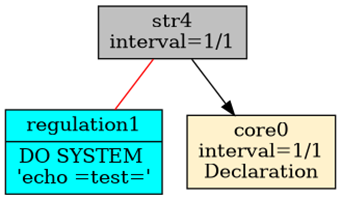
Fig. 9. Dependency between objects when using alerting
The image shows the relationship between the processes responsible for artifacts, alerting, and ephemerides. It should equally be possible to attach the process responsible for alerting to a substrate.
Alerting objects are shown in blue and connected, via red undirected lines, to the objects they monitor.
More than one alerting object can be attached. Multiple RULE commands can be associated with a given data-stream-creating command.
Looking more closely, we see that the process responsible for alerting is triggered by a condition. The following command lets us inspect what’s actually happening there:
$ xretractor -c query.rql -d -u -p > out.dot &&
dot -Tpng out.dot -o out.png
The output file looks as follows (Fig. 10):
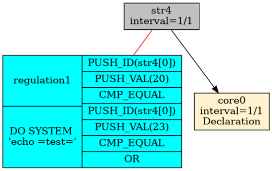
Fig. 10. Code responsible for the alerting trigger condition.
In its final form, this condition must evaluate to an expression representing true or false.
Logical Condition in RULE
The WHEN clause of the RULE command takes a logical expression, which is evaluated on every new record of the specified stream. If the expression evaluates to true, the process defined in the DO clause is triggered.
Comparison operators
| Operator | Meaning |
|---|---|
= | equal |
!= | not equal |
> | greater than |
< | less than |
>= | greater than or equal |
<= | less than or equal |
Logical connectives
| Operator | Meaning |
|---|---|
AND | conjunction - both conditions must be satisfied |
OR | disjunction - one condition is enough |
NOT | negation - the condition must not be satisfied |
A bare STRING field is true when its value is nonempty. String comparisons and NOT over a string return INTEGER 1 or 0. AND and OR use the left operand’s type, or the right operand’s type if the left is NULL; a result based on a string is INTEGER. Thus WHEN NOT status[0] is true for an empty string, and a false string comparison does not trigger a rule through OR. NULL still follows the condition’s three-valued logic.
Expression structure
A condition is built from the fields of the stream schema specified in the ON clause. Fields are identified the same way as in SELECT - by the stream name with an index:
WHEN stream[index] operator value
Compound conditions are joined with connectives:
WHEN stream[0] > 10 AND stream[1] != 0
WHEN stream[0] = 5 OR stream[0] = 7
WHEN NOT stream[0] < 0
Examples
RULE high_alarm \
ON measurements \
WHEN measurements[0] > 100 OR measurements[0] < -100 \
DO DUMP -10 TO 10 RETENTION 50

RULE signaling \
ON status \
WHEN status[0] = 1 AND status[1] != 0 \
DO SYSTEM 'systemctl restart sensor-reader'

RULE one_time ON data WHEN NOT data[0] = 0 DO DUMP -5 TO 0
Field access
The condition refers to the fields of the stream specified in ON. The field index corresponds to its position in that stream’s schema - the same as in the SELECT clause. The condition reads the stream’s output record, so an index equal to or greater than its field count is a compilation error (see Index out of range). Aliasing works exactly as described in the chapter Aliasing.
If the stream in ON was produced by an interleave A#B, the condition must use the output stream name:
RULE valid ON result WHEN result[0] > 0 DO DUMP -1 TO 0
A reference to a named interleave component is ambiguous and causes compilation to fail:
RULE invalid ON result WHEN A[0] > 0 DO DUMP -1 TO 0
The same rule applies when # is hidden in a substrate generated for a compound FROM expression.
Alerting Example
In a terminal window, we start the xretractor process, running the query.rql file shown at the start of the chapter.
$ xretractor query.rql
test
test
test
…
In a second terminal window, I suggest running the command:
$ xqry -s str4
27
28
20
21
22
23
24
25
26
27
I suggest placing both windows side by side. We will see that the appearance of the values 20 and 23 triggers the server-side action that prints “test”. Keep in mind that any system command or invocation of any program can appear here, depending on what we put in the DO SYSTEM declaration.
Session recording (animation below):
Animation. Session recording of the alerting example
Example 2: recording event context (DO DUMP)
The DO DUMP action lets you capture a window of samples surrounding an event - data before and after it occurred. This is useful when we want to preserve the context of an anomaly for later analysis.
We create a query.rql file:
STORAGE 'temp'

DECLARE a INTEGER STREAM core0, 1 TEXTFILE 'datafile1.txt'
SELECT str1[0] STREAM str1 FROM core0

RULE anomaly_log ON str1 WHEN str1[0] > 24 DO DUMP -3 TO 3
Input data - numbers from 20 to 28:
$ seq 20 28 > datafile1.txt
We run xretractor:
$ xretractor query.rql
When the value of stream str1 exceeds 24, the rule triggers a write of 6 records (3 historical + 3 subsequent) to the binary file temp/str1_anomaly_log_dump.tmp.
Reading the dump file
The dump file contains no .desc header - when opening it in xtrdb, the schema must be specified manually:
$ xtrdb
> storage temp
> open str1_anomaly_log_dump { INTEGER a }
> size
> list 6
> quit
The printed values are everything the file carries: a dump has no .meta file either, so NULL and a transmission gap have no representation in it, and a zero may be a genuine zero, a NULL field, or a record the engine did not have (→ Alerting implementation).
Example 3: rotating dumps (DO DUMP with RETENTION)
Without RETENTION, each successive trigger of the rule overwrites the same file. When events repeat, use RETENTION N to keep the last N dumps in separate files.
STORAGE 'temp'

DECLARE a INTEGER STREAM core0, 1 TEXTFILE 'datafile1.txt'
SELECT str1[0] STREAM str1 FROM core0

RULE anomaly_log ON str1 WHEN str1[0] > 24 DO DUMP -3 TO 3 RETENTION 5
Each trigger creates the next file (circular rotation):
temp/str1_anomaly_log_dump_0.tmp
temp/str1_anomaly_log_dump_1.tmp
temp/str1_anomaly_log_dump_2.tmp
temp/str1_anomaly_log_dump_3.tmp
temp/str1_anomaly_log_dump_4.tmp
Once capacity is exceeded (RETENTION 5), the oldest file is overwritten by the new one.
Example 4: multiple rules on a single stream
Any number of rules can be attached to a single stream. The example below combines both actions - a system notification and context recording:
STORAGE 'temp'

DECLARE a INTEGER STREAM core0, 1 TEXTFILE 'datafile1.txt'
SELECT str1[0] STREAM str1 FROM core0

RULE lower_threshold \
ON str1 \
WHEN str1[0] < 21 \
DO SYSTEM 'echo "ALARM: value below lower threshold" >> alarm.log'

RULE upper_threshold \
ON str1 \
WHEN str1[0] > 26 \
DO SYSTEM 'echo "ALARM: value above upper threshold" >> alarm.log'

RULE context_log ON str1 WHEN str1[0] > 26 DO DUMP -5 TO 5 RETENTION 10
The upper_threshold and context_log rules react to the same condition independently - crossing the upper threshold both writes a log entry and captures the data window at the same time. The lower_threshold rule handles the lower threshold separately.
All three rules are evaluated on every new sample of the str1 stream.
Configuration Directives
Four configuration directives are available:
- STORAGE
- SUBSTRAT
- ROTATION
- DEFAULT VOLATILE
STORAGE, SUBSTRAT, and ROTATION take a text argument in single quotes. DEFAULT VOLATILE takes no string. Example directives with arguments:
STORAGE 'temp_folder'
SUBSTRAT 'memory'
ROTATION 'rotation_counter.txt'
Fig. 11. Configuration directive syntax diagram
The railroad diagram in Fig. 11 was generated from the compiler_option and default_statement rules in the system’s ANTLR4 grammar (RQL.g4). The three upper branches (the compiler_option rule) have an identical structure: one of the keywords STORAGE, SUBSTRAT, or ROTATION (rounded green boxes), followed by a value enclosed in single quotes - arbitrary text (a directory path for STORAGE, a counter-file name for ROTATION), or the name of one of the predefined memory profiles (for SUBSTRAT). The bottom branch (the default_statement rule) is the keyword pair DEFAULT VOLATILE with no value.
The STORAGE directive selects the directory for output files. Without it, xretractor uses storage.dir from the TOML configuration, falling back to the process’s current directory only when that key is also unset. An explicit RQL directive takes precedence over configuration (see configuration file).
Substrates are queries and their effects that arise from the compiler decomposing system commands based on time-series algebra expressions. These are queries visible in the query execution plan but not specified directly in the .rql file. They arise from the implementation of the query-execution-plan construction process.
Without DEFAULT VOLATILE or explicit SUBSTRAT, such queries materialize data on disk in DEFAULT storage. Without retention their files grow without bound; the TOML key storage.default_retention can also limit substrate history. Keeping intermediate results on disk can be useful during software development, while SUBSTRAT 'memory' keeps only the history needed by the plan in a bounded RAM buffer.
The possible options for the SUBSTRAT command are: memory, default, direct, posix, posixshd, generic (case does not matter). Any other value is a compile error - including device and textsource, which are DECLARE source types, not storage profiles. A full description of each type - the C++ class, retention handling, and shadow support - can be found in the chapter Storage Types.
The last directive - Rotation - indicates an alternative shutdown mode for the system. By default, after compilation, all files produced by the system remain in whatever state the system left the recorded data. On the next invocation of the system command, all artifact and substrate files are deleted. Using the Rotation directive in an rql file containing query declarations makes the system create the file named in the directive’s parameter and store there a counter incremented on every system startup. Artifact and substrate files are renamed at the end of every system run - they get an .old extension plus a number derived from the increasing counter. This process is called artifact rotation.
DEFAULT VOLATILE
DEFAULT VOLATILE
This directive (the default_statement rule) selects default in-memory storage for both named SELECT results and compiler-generated substrates. It may appear once in the header, before DECLARE, SELECT, and RULE. Explicit SUBSTRAT takes precedence for substrates; PERSISTENT or explicit STORAGE on a SELECT overrides the default for its result. DECLARE sources remain unchanged. For examples and the complete rules, see VOLATILE and PERSISTENT.
System Architecture
The construction of the data-processing system is a strictly technical chapter. Here I present how the system was designed and built, and where and how its functionality is currently laid out.
RetractorDB was implemented in C++ under Linux. The source code goes through continuous integration and testing on GitHub, backed by CircleCI. The code is run and developed locally on the Linux WSL2 platform. I abandoned development and implementation of the system under Windows. In the early phase I kept that option open, and I may return to it in the future. However, maintaining too many development platforms significantly slows down rapid prototyping and system development. I still keep and maintain the system’s functionality on the Linux ARM platform. The code is compiled and tested on ARM and x86-64 architecture machines running in CircleCI’s resources. Raspberry Pi is one of the intended production platforms for RetractorDB, aimed at Edge IoT needs.
The build uses Conan 2, CMake, and Ninja. Tool preparation, source builds, and release-package installation are described in Installation Process. Linux remains the general deployment contract of this manual; the Apple port is solely for development and testing, with its limitations covered in a separate section of that appendix.
Overview of topics covered in this chapter
The chapter is built in layers - from the general view down to implementation detail.
-
The system as a trio of cooperating programs:
xretractoras the process executing a query plan,xqryas the multi-instance client for current data, andxtrdbas the binary-file inspection tool. Several namedxretractorprocesses can run on one host, each with its own Boost IPC area. The diagram in Fig. 12 shows component boundaries for one such instance. -
Multiple Instances and the Bus
Instance names, separation of IPC objects, the
xrdbbusregistry, global protection of stream and storage-file names, and automatic routing rules forxqrycommands. This section also describes the stableserviceidentity, complete plan replacement withxqry --reset, and the modes shown byxqry --bus. -
Which data paths are always active (data arrival → xretractor → artifacts), and which are optional or diagnostic. The graceful-shutdown mechanism is also described - xretractor reacts to
SIGINT,SIGTERM, andSIGHUPsignals by finishing the current cycle without risking file corruption. -
Artifacts, Substrates, and Ephemerides
The system’s key taxonomic split. Each stream type has a different purpose and a different storage strategy: artifacts are materialized on disk as a durable result, substrates are intermediate streams necessary during computation, and ephemerides are ephemeral data sources that cannot, or need not, be stored.
-
The four-file structure of an artifact: a binary data file (fixed-length records, no header), a
.descdescriptor describing the record schema in ANTLR4 grammar, a.metametadata file with an index of null values and transmission gaps (RLE encoding), and an optional.shadowfile for non-destructive modification of historical records. The descriptor determines the storage strategy via theTYPEfield. -
Compilation and Plan Construction
The process of turning an
.rqlfile into a ready-to-run query execution plan. The-cflag runs compile-only mode without execution; combined with-d -f -sit generates DOT output, whichgraphvizturns into a data-flow graph. The graph shows two domains: the arithmetic-expression stack (PUSH, ADD, etc.) and the stream algebra. The full set of compile-mode and execution-mode flags is described. -
Data Processing and Distribution
A complete walkthrough: from preparing a data file, through running
xretractor, through viewing streaming statistics (xqry -d), to live visualization in gnuplot (xqry -s str1 -p 50,50 | gnuplot) and network transmission vianc. The example combines two sources - a text file and/dev/urandom- illustrating how the+operator in the FROM clause performs algebraic stream joining. -
The
xtrdbtool - an interactive binary-file inspector modeled after the dbase style. The.open,.desc,.list,.rlist, and.metacommands let you browse the contents of artifacts without knowing the binary format. The tool is also used to verify determinism: the same input data should always produce identical results.
Three commands are enough to run a complete pipeline:
xretractor -c query.rql          # verify the query file's correctness
xretractor query.rql             # start processing
xqry -s <stream>                 # read current data
A fourth element - xtrdb - comes into play for diagnostics and testing, not in a typical production workflow.
General Perspective
The system is built around 3 programs available as system commands. The first is the compiler and query-plan execution engine. The second is the client for accessing current data. The third is the program that provides access to binary dumps. Their names are, in order:
- xretractor
- xqry
- xtrdb
The xretractor program creates a process that executes one independent RetractorDB plan. Several named instances can run on a host, each with its own shared-memory area. The xqry program creates processes that communicate with a selected instance, while a shared bus enables discovery and routing. The xtrdb program is used to analyze data and metadata stored in the database’s files.
Below, Fig. 12 schematically shows RetractorDB’s architecture. All currently existing components are included. The areas enclosed in boxes with headers filled with system commands correspond to the existing components. The artifact-storage area is a symbolic representation of the filesystem.

Fig. 12. Data-flow diagram between RetractorDB processes
In Fig. 12 we see the processes carried out by the xretractor, xtrdb, and xqry programs. The figure presents one execution instance; in a multi-server deployment, the xretractor block together with its IPC and clients is repeated for every name. Relationships between instances are described in Multiple Instances and the Bus.
An xretractor process communicates with xqry processes through its own named shared-memory area. In this memory, a data queue is created for every xqry subscription. Data is received by xqry processes on an ongoing basis. The job of the xqry processes is to forward the data on to other systems or processes. If an xqry process dies or is terminated, the relevant xretractor instance frees the resources dedicated to that client.
Besides directing data for delivery through shared memory, RetractorDB also writes data to the so-called artifact-storage area. Currently this is a directory to which the results of the stream-processing carried out according to RetractorDB’s query execution plans are continuously written.
⚠️ Warning
The “Database” shown in the figure is not a relational database. By “database” in the figure shown, we mean a set of binary or text files managed by RetractorDB. Data is pulled from devices and written to rotating or non-rotating binary or text files. Access to this data is carried out via the xtrdb tool, or, while the system is running, via the xqry process.
The file with RQL queries and directives is given as the first argument to the command that starts the system. That argument is optional: invoking xretractor without a query file starts it in idle mode - the process comes up, takes the service lock, opens the IPC channel and waits, building neither a plan nor a timeline. This lets a systemd unit come up together with the operating system, before the operator supplies a query set. The exception is --onlycompile mode, where a missing file remains an error - there is nothing to compile.
A query set can be supplied later in three ways. xqry -a adds one SELECT, DECLARE, or RULE to an active plan. xqry --reset file.rql atomically replaces the complete plan without restarting the process and can start the first epoch of an idle instance. Running xretractor file.rql while the service is live can instead validate the file, store it as the startup plan, and restart the systemd unit. The latter two routes accept a complete set including :STORAGE, :SUBSTRAT, and :ROTATION directives.
NOTE: Idle mode is covered by the
service_idletest (variants using the--serviceflag and theXRETRACTOR_SERVICEenvironment variable).
Multiple Instances and the Bus
Several xretractor processes can run concurrently on one host. Each instance has its own name, lock, IPC area, plan, and clients. The shared xrdbbus bus registers live instances, lets xqry discover them, and ensures that two plans do not claim resources that cannot be shared safely.

Fig. 13. Concurrent instances and the shared xrdbbus bus
In Fig. 13 every instance compiles its own plan and claims its own set of stream names in a bus slot; numbered nodes stand in for the names there, because all that matters is that they never repeat across instances. What is disjoint are the object names, not the memory area: on Linux the bus segment and the IPC objects of every instance live in the same /dev/shm and differ only by the instance-name suffix - for instance alpha these are the command queue RetractorQueryQueue.alpha, the response segment RetractorReply_v1.alpha, and the client subscription queue brcdbr.alpha.<pid>. The response segment has fixed slots and atomic states; it does not use a separate named map mutex. The storage directory is shared as well, with the files of the individual instances kept disjoint.
Service mode is the exception: exactly one instance may be marked as the service in the host’s default namespace. By default it receives the stable name service, so scripts can address --server service without first inspecting the bus.
Instance identity
An instance can be identified in three ways:
| Mechanism | Meaning |
|---|---|
xretractor --name measurements plan.rql | A stable name supplied by the operator. |
xretractor --autoname plan.rql | A random, container-style name printed at startup. |
server.autoname = true | Automatic naming from the TOML file, unless --name was given. |
An explicit --name takes precedence over configuration. A name must match [a-z][a-z0-9_-]* and may contain at most 32 characters. --name and --autoname are mutually exclusive.
Omitting the name preserves the historical identity: IPC object names and the lock file have no suffix. This instance is also published on the bus, as (unnamed), and takes part in collision checks.
The RDB_NAMESPACE environment variable selects a separate bus segment and, when neither --name nor --autoname is given, becomes the default server name and xqry target. It is used primarily by parallel integration tests. Explicit --name, --autoname, and --server options still take precedence. The one-service limit is enforced separately in each bus namespace. Different RDB_NAMESPACE values with the same explicit server name do not separate IPC objects: their names follow the selected instance identity.
Before startup, an instance acquires its file lock in paths.lock_dir (the temporary directory by default) and an additional IPC identity lock at /tmp/xretractor_ipc.<command-queue-name>.lock. The latter location is fixed, independently of TMPDIR and paths.lock_dir. A held IPC identity blocks startup before artifacts are removed or IPC is created, even if the bus is unavailable. Changing the lock directory or bus namespace does not allow taking over a live server’s objects.
Private and shared resources
Named instances have separate Boost.Interprocess objects. The base names of the command queue and response segment receive the instance suffix; a subscriber queue also contains the client PID. Stopping an instance ends only its subscriptions and removes its IPC; it may also clean up resources abandoned by dead processes. Live instances remain protected.
New IPC objects created by the server receive an explicit 0600 mode, which restricts access to the server account without relying on the process umask. This applies to the command queue, subscription queues, response segment, and bus segment. Separate names keep the resources of cooperating instances apart, and locks coordinate their creation and cleanup.
The fix for #465 creates command queues, subscription queues, and the response segment through create_only. A name collision does not lead to adopting an existing object. When opening a queue or segment, the server and client require its owner to match their own effective UID (geteuid()) and its mode to be exactly 0600. The expected UID comes from the process credentials, not from the metadata of the object being opened. Before mapping, the checks also cover object type, a single link, agreement between the name and the opened object, and directory protection against entry substitution by another account.
At startup or restart, the server may remove leftovers owned by its own account after acquiring the IPC identity lock; older, broader permissions on such an object do not prevent cleanup. Resubscription removes the previous queue belonging to that account and creates a new one with the requested capacity. Cleanup refuses to remove an object owned by a different UID, including when performed by root. Abandoned locks belonging to other accounts are skipped, and identity and presence locks continue to protect live instances. The abandoned-resource sweeper does not enumerate all subscription queues left after SIGKILL.
A refusal is logged at ERROR level, including in Release, with the object name, reason, and owner UID when it can be determined. A foreign command queue or response segment refuses startup; a foreign subscription queue refuses that subscription. The bus may open an existing segment only after the same verification, and a rejected segment remains untouched. Its unavailability retains the single-server fallback described below.
⚠️ Warning
xqrymust run with the same effective UID as the server. This also applies to administrators: running the client as root alone does not allow it to open IPC owned by another service account. For a service running asretractor, use, for example,sudo -u retractor xqry --server service --dir. Sharing the bus requires the same UID; an instance name orRDB_NAMESPACEdoes not replace owner verification. AllowingSYSTEMrules in a replacement plan still depends onservice.unrestricted(see xqry).
The bus is shared by the host or RDB_NAMESPACE. Every live server publishes its name, PID, operating modes, plan file, and stream names. When the process entry is readable, a slot remains live if its PID and nonzero start time match; a zombie process does not retain resources. On Linux the engine reads /proc/<pid>/task/<pid>/stat, while on macOS it uses the platform adapter.
An unreadable process entry means the engine cannot decide, rather than confirming that the owner is dead. On Linux a failed read confirms absence only when kill(pid, 0) returns ESRCH; success or EPERM leaves the result uncertain. bus::isProcessAlive() then keeps the slot and its claims, including when it cannot compare start times. This protects an owner hidden by hidepid or ProtectProc, but may retain stale claims after PID reuse. Lack of access to an entry alone therefore does not authorize releasing resources. The rule is checked by ut_bus::BusFixture.UnreadableOwnerKeepsSlot.
The current layout uses the xrdbbus_v7 segment, or xrdbbus_v7_<RDB_NAMESPACE> when RDB_NAMESPACE is set. Each namespace has its own registry and collision checks. Segment users hold a presence lock through flock; the last one leaving can remove the unused segment. Layout versions have separate registries: concurrently running binaries using v6 and v7 does not provide collision checks between their streams and storage paths. Stop older instances before upgrading.
Shared presence-lock acquisition retries nonblocking flock calls for up to 500 ms. A transient exclusive holder may release its lock within that period; if it still holds it, the bus remains unavailable instead of blocking attachment indefinitely. This deadline applies to waiting for flock, not to the entire file-opening procedure.
Before starting or replacing a plan, the bus checks that the following do not overlap:
- all stream names, including compiler-generated and ad hoc streams;
- normalized paths of storage files being written;
- the counter file of the
:ROTATIONdirective.
Resources are claimed before old artifacts are removed and before IPC is created. A losing instance therefore cannot delete data belonging to a live owner. The rejection message identifies the conflicting resource, instance name, and PID.
For xqry --reset, the new plan’s resources are reserved first. Only after the new epoch has been built successfully does that reservation atomically replace the active set. A parse error, compilation error, limit error, or collision leaves the current plan and its claims unchanged.
An unrecoverable bus-mutex error, ENOTRECOVERABLE, is reported at ERROR level, including in Release, once per Bus object. The message identifies the /dev/shm segment to remove after all instances mapping it have stopped. Removing a segment still used by a live instance can split the resource registry. Startup and ad hoc import retain the emergency mode described below; plan replacement is rejected when an attached bus has an unusable mutex.
⚠️ Warning
An unavailable or corrupted bus does not stop an individual server if it can acquire its instance and IPC identity locks. Startup is allowed with a warning, but global stream-name and storage-path protection is then not enforced. The IPC identity lock still applies. This is an emergency mode, not a valid multi-server configuration.
Routing xqry commands
xqry resolves its target from a single snapshot of the bus in the current RDB_NAMESPACE, without probing servers in turn or waiting for their timeouts. The combined --bus listing does not expand the routing scope of other commands.
| Situation | Result |
|---|---|
--server name was given | The named instance is used without automatic routing. |
| Exactly one instance is live | The client selects it automatically. |
Several instances, --select or --detail | The stream owner is selected. |
Several instances, ad hoc SELECT | All sources must belong to one instance. |
Several instances, ad hoc RULE | The owner of the stream in the ON clause is selected. |
Several instances, ad hoc DECLARE | --server is required because the declaration has no input owner. |
| Several instances, instance-wide command | --hello, --dir, --kill, and --reset require --server. |
An ad hoc query cannot combine sources from different instances. RetractorDB does not transfer streams between servers; the plans remain independent execution graphs.
Inspecting the bus
xqry --bus does not contact any server. Without setting RDB_NAMESPACE, it discovers every bus of the current version that is accessible to the current account and has live instances. Each bus gets a separate NAMESPACE: section with instance names, PIDs, modes, query files, and streams; (default) denotes the bus without a namespace. The --yaml modifier produces one apiVersion: xqry/v1 document with a servers list. Every entry has a namespace field: null for the default bus or a quoted namespace name. With no live instances, table output is empty and YAML contains servers: [].
The MODE column can contain several letters:
| Letter | Mode |
|---|---|
N | normal clock-paced execution |
R | --realtime |
F | --no-clock |
U | --until-eof |
M | --llimitqry is set |
X | --xqrywait |
S | service mode or a systemd unit |
Example session:
xretractor alpha.rql --name alpha --noanykey &
xretractor beta.rql --name beta --noanykey &

xqry --bus
xqry --select temperature         # routed by stream owner
xqry --server alpha --dir         # explicit instance-wide command
xqry --server beta --kill         # stops only the beta instance
Data and Control Flow
Data and control in RetractorDB give rise to several potential ways of using the system’s components. Fig. 14 schematically shows the flow of data between RetractorDB’s processes, Linux system processes, and the source data and results produced by each process.
The thickest lines represent the flow that is always present when regular time series are processed. After receiving an .rql file, xretractor compiles it, builds the query-plan tree, begins processing incoming data, and creates binary files containing artifacts. Without a file it can start idle and wait for a complete plan delivered by xqry --reset.
NOTE: The functionality described here is covered by the test:
consistency, described in the appendix Integration Tests.
To control the xretractor process once it has started, we use the xqry process. Through it, we can stop the xretractor process, retrieve statistics, or request access to current data.
The remaining arrows represent data flows that depend on the specific process being carried out with RetractorDB. Dashed arrows are typically intended for diagnostic purposes.
Each process on the diagram is additionally labeled with the number of continuous processes of that kind maintained in the system. The historical label “1” next to xretractor describes the one plan instance shown in the figure, not the current host-wide limit. Named instances can run concurrently; exactly one may act as the service in the default host namespace. The xrdbbus bus enforces separation of their resources. The xtrdb program does not maintain a continuous process: it reads data, returns a result, and exits, or runs interactively. The xqry process is labeled “N” because several clients can connect to each xretractor instance.

Fig. 14. Data and control flow
Stopping xretractor
The xretractor process handles system signals and shuts down in a controlled manner upon receiving:
| Signal | Command | Meaning |
|---|---|---|
SIGINT | Ctrl+C in a terminal | interactive interrupt |
SIGTERM | kill <pid> | standard process termination |
SIGHUP | kill -HUP <pid> | termination on terminal close |
All three signals produce the same effect: a graceful shutdown - the processing loop finishes the current cycle and stops. A signal that finds the loop waiting for the deadline of the next slot ends it immediately, and the slot whose deadline has not yet come is no longer computed (see Slot schedule). This allows xretractor, running as a service, to be shut down safely without risking corruption of artifact files.
Stopping via xqry
Besides system signals, xretractor can be stopped programmatically - using the command:
xqry --server name --kill
How the shutdown proceeds step by step
1. xqry sends a “kill” request
The xqry process resolves an instance from --server or from the bus, builds an IPC message, and places it on that instance’s command queue. The base name RetractorQueryQueue receives the named-instance suffix. The message contains the xqry process’s identifier (PID) and the kill command.
2. xretractor receives the command and sets the stop flag
The selected instance’s IpcServer communication thread continuously listens on its queue. After receiving a kill message, executorsm::commandProcessor sets the atomic iLoopLimitCnt counter to stop_now and wakes the execution loop. The same mechanism is used by the system-signal handler - regardless of the source, the effect is identical for that one instance.
3. The main processing loop detects the flag and finishes the current cycle
The main loop checks iLoopLimitCnt on every iteration. When it detects the value stop_now, it finishes the current cycle and exits the loop - without interrupting mid-computation. This ensures the integrity of the artifacts being written.
4. xretractor notifies all connected clients (OOB broadcast)
After exiting the loop, xretractor calls IpcServer::broadcastOutOfBusiness(). The IPC object walks the subscription registry, where the show command stored each client’s PID and stream name. It sends every registered client a special OUT_OF_BUSSINESS message on its dedicated queue.
5. Every xqry client receives the termination signal and exits
Every xqry subscription has its own queue containing the server name and client PID. Upon receiving the OUT_OF_BUSSINESS message, xqry sets its internal done flag and shuts down in a controlled manner - regardless of how much data it had received up to that point.
6. IPC resource cleanup
Finally, xretractor removes its response segment, command queue, mutex, and client queues, and releases its bus slot and locks. The owner removes lock files before releasing their locks. Additional cleanup at exit removes accessible resources abandoned by dead instances; live processes remain untouched. The last user of a bus segment can remove it after acquiring the exclusive presence lock.
After SIGKILL, exit handlers do not run and resources may remain. xretractor --cleanup removes recognized leftovers without starting a plan. Its scope, limitations, and counters are described in the xretractor options. It does not remove client response queues or older bus-layout segments.
Fatal errors and emergency cleanup
A fatal error during startup or in the communication thread follows the same final resource ownership policy but does not attempt to continue the processing cycle. The spdlog registry is flushed rather than destroyed before atexit handlers run. If the error originated in the communication thread itself, cleanup detaches that thread instead of attempting to join it from itself. It then removes IPC queues and shared memory and releases the service lock last.
The process exits with status 1. A later start therefore finds neither orphaned IPC nor a stale service lock, and the primary failure is not masked by a secondary SIGSEGV or SIGABRT during shutdown.
NOTE:
fatal_exit_pathcovers both startup failure and failure reported by the communication thread.
What happens with multiple xqry processes
RetractorDB is designed to work with multiple parallel clients. If, say, three xqry processes are running simultaneously, subscribed to different streams, and one of them calls xqry --kill:
- the selected xretractor processes the kill request once, regardless of which client sent it,
IpcServer::broadcastOutOfBusiness()sends theOUT_OF_BUSSINESSmessage to all clients registered with that instance,- each of the three xqry processes receives the termination signal and exits on its own,
- clients that hadn’t subscribed to any stream (e.g. xqry invoked only with
--diror--hello) are not entered in the map and don’t need to be notified - these commands exit immediately after providing their response.
Clients connected to other named instances do not receive the message and continue running.
It’s worth noting that xqry also detects server inactivity: if no data arrives for 10 seconds, the client shuts itself down with a warning in the log. This is a safeguard in case xretractor crashes suddenly without being able to send the OOB message.
Artifacts, Substrates, Ephemerides
Given that the system is designed for continuous operation, and that, theoretically, the results obtained without a data-retention process would fill up any storage medium, we introduce additional definitions related to the nature of the data being processed.
In presenting the description of Fig. 14, artifacts were mentioned. This is one of the terms that needs explaining.
✅ Note
Definition (Artifact): By artifacts we mean data processed in the system in the form of streams that are ultimately materialized as a durable result and effect of processing other data.
Continuous time series can be read from devices, then processed - reduced or resized in time and in dimension. But as a rule, certain data should be saved. Whether that data is later subject to retention is a secondary matter. Data that constitutes the result and expected output of the system, we call artifacts. Something we expect and materialize for the end user’s needs.
✅ Note
Definition (Substrate): Substrates are intermediate objects. As a result of processing time series, data streams may arise that are ephemeral - needed only for and during processing.
Their size can be significant, considering how far back we go, for example when dumping historical monitoring data. However, their existence is irrelevant with respect to the system’s desired output. We call such data streams substrates. They arise as a result of the system’s operation; as a rule they do not appear explicitly in queries - but they result from the process of processing time series, and yet their results are necessary to accomplish the task.
✅ Note
Definition (Ephemeris): Ephemerides are objects on the basis of which we create source data streams - data that cannot be stored. As a rule, these are ephemeral, transient data.
For example, the system reads random numbers at a given rate, and it is precisely this data source that provides ephemeral data. It cannot be returned; storing it is, as a rule, pointless - it must be passed on for further processing in order to produce artifacts or substrates, and then discarded and replaced with new, current data.
Data Storage Format
The system processes time series in three forms: artifacts, ephemerides, and substrates. Each type has a different purpose and a different storage strategy.
Substrates and Artifacts are formally no different in the system. The only difference is that substrates were generated based on data-stream algebra equations and were not written directly in the sequence of commands given to the compiler. If we declare an Artifact stream that covers what would otherwise be a substrate, the substrate is eliminated. Ephemerides are streams created via the Declare command - they contain values that exist only briefly.
Storage accessor types
NOTE: The functionality described here is covered by the test:
txtsrc, described in the appendix Integration Tests.
The TYPE field in the descriptor (or the STORAGE directive in RQL) selects the FileInterface implementation:
Type (TYPE_PROFILE) | Implementation class | Purpose |
|---|---|---|
DEFAULT | groupFile<posixBinaryFileWithShadow> | Default artifacts - data file + shadow file, with retention |
DIRECT | groupFile<posixBinaryFile> | Direct writes without shadow, with retention |
POSIX | posixBinaryFile | Raw POSIX write, no shadow |
POSIXSHD | posixBinaryFileWithShadow | POSIX with a shadow file |
MEMORY | memoryFile | RAM-only storage (ephemerides) |
GENERIC | genericBinaryFile | Generic binary accessor |
BINFILE | binaryDeviceRO | Regular binary input-data file, DECLARE ... BINFILE (read-only) |
DEVICE | binaryDeviceRO | Character device or FIFO, DECLARE ... DEVICE (read-only) |
TEXTSOURCE | textSourceRO | Text input-data source, DECLARE ... TEXTFILE (read-only) |
The artifact and substrate file set
Artifacts and substrates written to disk can be associated with up to five files:
| File | Extension | Purpose |
|---|---|---|
| Binary data file | (stream name) | The main record stream - append-only |
| Descriptor file | .desc | Record schema (fields, types, sizes, storage type) |
| Metadata file | .meta | Index of null values and transmission gaps (RLE) |
| Data shadow file | .shadow | Record modifications without overwriting original data |
| Index shadow file | .meta.shadow | Null-pattern overrides accompanying .shadow |
%% pdf-width: 70%
graph TD
  D[".desc: descriptor (record schema)"]
  B["Binary data file (N×R-byte records)"]
  M[".meta: metadata (null and gap index)"]
  S[".shadow: data shadow file (record modifications)"]
  MS[".meta.shadow: index shadow (null overrides)"]

    D -->|"describes structure"| B
    B -->|"companion index"| M
    B -->|"optional overrides"| S
    S -.->|"consistency pair"| MS
    M -->|"pattern overrides"| MS

    style S fill:#f9c,color:#000
    style MS fill:#f9c,color:#000
    style M fill:#cdf,color:#000
Fig. 15. The artifact file set and their relationships
The diagram in Fig. 15 shows the static relationship between artifact files: .desc defines the record structure, .meta indexes nulls and gaps, .shadow stores optional record overrides, and .meta.shadow the null-pattern overrides that correspond to them. The two shadow files always go together.
The shadow files and the metadata file are optional. With continuous, gap-free, unmodified data arrival, the binary data file and the descriptor alone are enough.
Ephemerides have no data file of their own - their source is an external object (a text file, a device) that the system neither creates nor deletes. A .desc descriptor describing the read schema is created for them, however. No .meta index appears: declared sources get an inert metadata-index variant that works purely in memory.
The dump file produced by a DO DUMP rule does not belong to this set, although its records have the same layout. No .desc, no .meta and no header accompany it, so it carries values only: the information about NULL and about a transmission gap stays inside the engine and never reaches the dump. The dump contract is described in Alerting implementation.
Chapters
- Artifact Files - descriptor, binary data, metadata, shadow file, and the relationships between them
- File Rotation Mechanism - the
ROTATIONdirective, file lifecycle, session examples - Inspection Tool
xtrdb -s- the storage map, report sections, examples - Summary - rationale for the chosen structure, comparison of approaches
Files
This chapter describes the five files that make up the complete file set of an artifact or substrate: the schema descriptor (.desc), the main binary data file, the metadata index (.meta), the data shadow file (.shadow), and the index shadow file (.meta.shadow). For each file, the binary format, field semantics, and read/write rules are presented. The chapter also covers the metaData class - the RLE compression mechanism, transmission-gap handling, the update interface, and persistence across restarts. The final section shows the relationships between all the files at the level of append, update, and read operations.
The scope of this chapter does not include the file-rotation mechanism between sessions (→ Rotation) or the xtrdb -s inspection tool (→ Inspection Tool).
File opens and symbolic links
Storage files - data, .shadow, .meta, .meta.shadow, and .desc - are opened with O_NOFOLLOW: a symbolic link at the final filename causes the open to be refused instead of writing to or truncating its target. For GENERIC, refusal may occur only at the first write. An unavailable metadata index may disable its persistence without stopping the stream; refusal to open a link therefore does not always mean rejection of the entire plan.
The exception is the main data file named by an explicit REF supplied by the caller (a plan or a schema in xtrdb). That operator choice can authorize a final data-file link. A REF read only from an existing .desc does not grant this permission, nor does allowing a directory through storage.ref_dirs. The exception covers neither auxiliary files nor retention-segment names generated by the engine.
O_NOFOLLOW checks only the last path component. The storage directory and its ancestors may still be links; replacement of a parent directory during path resolution remains outside this guarantee. ut_rdb checks refusals and permitted controls. DUMP files have a separate policy that removes the final entry and exclusively creates a new file - see Alerting Implementation.
The descriptor file (.desc)
The .desc file describes the record structure. It is parsed by an ANTLR4 grammar (DESC.g4) and can contain data fields, storage-type meta-information, and a retention policy.
Syntax
{ <statement>* }
Each statement is one of the following:
BYTE     name [N]          # array of N bytes (default N=1)
INTEGER  name [N]          # 32-bit signed integers
UINT     name [N]          # 32-bit unsigned
FLOAT    name [N]          # 32-bit floating point (IEEE 754)
DOUBLE   name [N]          # 64-bit floating point
RATIONAL name [N]          # pair of int32: numerator and denominator
STRING   name [size]       # fixed-length string
REF      "path/file"       # data file (relative paths use the process's working directory)
TYPE     identifier        # storage type (DEFAULT, MEMORY, POSIXSHD, …)
RETENTION capacity segment # cyclic on-disk retention
RETMEMORY capacity         # cyclic in-memory retention
Example .desc files
A default artifact - two numeric fields, DEFAULT storage (data file + shadow file):
{
  INTEGER  ts
  FLOAT    value
  TYPE     DEFAULT
}
A SELECT result or substrate in RAM - MEMORY storage with a one-record ring (ephemeris sources declared with DECLARE have type BINFILE, TEXTSOURCE, or DEVICE):
{
  DOUBLE   x
  DOUBLE   y
  TYPE     MEMORY
  RETMEMORY 1
}
A substrate with retention - up to 1000 records on disk (10 segments of 100):
{
  INTEGER  ts
  FLOAT    a
  FLOAT    b
  TYPE     DEFAULT
  RETENTION 100 10
}
A binary source declaration (DECLARE in RQL generates this schema):
{
  INTEGER  a
  FLOAT    b
  TYPE     BINFILE
  REF      "sensor/data.bin"
}
Field type sizes
| Type | Size of a single value |
|---|---|
BYTE | 1 B |
INTEGER | 4 B |
UINT | 4 B |
FLOAT | 4 B |
DOUBLE | 8 B |
RATIONAL | 8 B (two int32) |
STRING | N B (declared size) |
For array fields name[N], the total size = type_size × N. The TYPE, REF, RETENTION, and RETMEMORY fields take no space in the record - they are descriptor metadata.
Record size R = the sum of the sizes of all data fields.
The RATIONAL field layout
A RATIONAL field stores a rational number as a pair of signed integers, written into the record directly, with no header and no type tag:
offset +0   int32   numerator
offset +4   int32   denominator
The byte order is the machine’s native one - little-endian on x86-64 and ARM64, the same as for INTEGER and UINT fields. The field occupies 8 bytes; in an array field RATIONAL name[N] the pairs follow one another, 8 × N bytes in total.
The value is always stored in lowest terms, and the denominator is always positive - the sign is carried by the numerator alone. This follows from boost::rational arithmetic, which normalizes the result on every assignment; it is not a writing convention. In particular:
- zero is stored as
0/1, never as0/0or0/5; - a whole number is stored as
n/1- aRATIONALfield with denominator 1 is exactly an integer, with no rounding involved (the slot-divisibility test in the query tree traversal algorithm relies on the same invariant); - the denominator is never zero - no write path in the system produces such a pair.
The invariant describes writing, however, not every file that can be handed to the engine. Since 23 September 2026 the read path checks it at the bytes-to-value boundary: a pair whose denominator is less than or equal to zero yields NULL, not a rational number. This covers a zeroed record (0/0), a denominator equal to INT_MIN, and the pair INT_MIN/-1 - exactly the bytes on which the previous version terminated the process with SIGFPE. A pair with a positive denominator also passes through normalization, so a reducible representation comes back reduced (2/4 as 1/2). The pair 1/-2 yields NULL because its denominator is negative. For a file written by the system this changes nothing - it contains no such pairs.
RATIONAL fields are produced by the MIN, MAX, AVG, and SUMC reducers when the input value has type BYTE, INTEGER, UINT, or RATIONAL. This covers current-record reducers in FROM, the deprecated .min/.max/.avg/.sumc notation, and record-history AGG(expression : W) in the SELECT list. FLOAT and DOUBLE inputs preserve their types (→ Aggregate Operators). A reducer over integer or rational input is, in practice, the main source of RATIONAL in an artifact.
A measured example
A plan computing the mean over a window of three samples:
DECLARE v INTEGER STREAM src, 1 TEXTFILE 'data.txt'

SELECT * STREAM ravg FROM AVG(src@(1,3))
fed with -3, -3, -2, 7, 7, 7, … yields the descriptor { RATIONAL avg } and a data file whose first record is eight bytes long:
f8 ff ff ff   03 00 00 00
└ numerator ┘ └ denominator ┘
   -8              3            →  -8/3
The fourth record is 07 00 00 00 01 00 00 00, that is 7/1 - the mean of three sevens, stored as a rational number with denominator 1 rather than as an INTEGER.
Reading the value without decoding bytes
The pair layout only matters when reading the binary file directly. That a field is of type RATIONAL and occupies 8 bytes is reported by xtrdb -s name from the descriptor (→ Inspection Tool) - the tool shows structure, not values. The value itself is obtained by passing the field through a conversion in the query; three functions offer three different trade-offs:
| Written in SELECT | Result for -8/3 | Note |
|---|---|---|
to_string(field : N) | the text -8/3 in a STRING[N] field | exact form; a whole number comes out as 7/1, not 7 |
to_double(field) | a DOUBLE field holding -2.6666… | an approximation, but sign and magnitude are preserved |
to_integer(field) | an INTEGER field holding -2 | truncation toward zero, not floor - → Field Expressions and Scalar Functions |
For export to text-based systems to_string is the right choice, because it preserves the value exactly; to_integer is convenient but drops the fractional part, and does so differently from Python’s flooring // - the rounding rule is documented alongside the expression functions.
The TYPE field and storage strategy
The TYPE field in the descriptor directly determines which accessor (FileInterface) is used by storage::initializeAccessor(). The absence of a TYPE field is equivalent to DEFAULT. The value is case-insensitive (MEMORY = memory).
The binary data file
The data file is a sequence of fixed-length records, written one after another with no header at all. The size of a single record R is determined by the descriptor as the sum of all field sizes in bytes.
| Offset in file | Content | Size |
|---|---|---|
| 0 | Record 0 | R bytes |
| R | Record 1 | R bytes |
| 2R | Record 2 | R bytes |
| … | … | … |
| (N-1) × R | Record N-1 | R bytes |
Every record contains the packed field values in the order defined by the descriptor:
| Offset in record | Field | Size |
|---|---|---|
| 0 | field_0 | len_0 bytes |
| len_0 | field_1 | len_1 bytes |
| len_0 + len_1 | … | … |
| len_0 + len_1 + … + len_n | field_n | len_n bytes |
The append operation (adding a new record) writes data to the end of the file. The update operation (modifying an existing record) - if a shadow file exists - goes into the shadow file, not the main file.
Example
DECLARE a INTEGER, b FLOAT STREAM src, 0.1 BINFILE 'data.dat'
SELECT * STREAM str1 FROM src
Record size: INTEGER (4 B) + FLOAT (4 B) = 8 bytes. After 50 records have been written, the output file str1 occupies 50 x 8 = 400 bytes. With a 0.1 s interval, this represents 5 seconds of data. data.dat is an existing read-only source; DECLARE does not grow it.
Reading a record that does not exist
A request for an index past the last record - or a read from an empty store - is not a successful read. Since 23 September 2026 storage::read() and storage::revRead() return a separate NoSuchRecord status, zero the destination buffer, and set the entire null pattern to true: a record that does not exist is an undetermined value, not a zero record. This is the same convention dataModel::fetchBack() and fetchForward() apply to a read beyond the accumulated history.
This matters for the result, not only for diagnostics. Previously that branch returned success and marked the zeroed record explicitly as not null, so NULL absorption did not kick in and the MIN, MAX, SUMC, and AVG reducers folded a fabricated zero into the result instead of skipping the missing record (→ Aggregate Operators). The xtrdb tool distinguishes an initial out-of-range refusal (record out of range, with no payload change) from a failed read of an allowed index (error and, for a list, fetch error). See xtrdb for details.
The null pattern lives in the payload and in the .meta index, that is, inside the engine. A DO DUMP dump does not carry it - a non-existent record is written there as zeros indistinguishable from data (→ Alerting implementation).
The metadata file (.meta)
The .meta file is an index of null values and transmission gaps. It stores information about which record fields have null values, and where gaps occurred - without duplicating the data itself.
File format
| Position | Content | Size |
|---|---|---|
| Header | reserved field (int64, always 0) | 8 bytes |
| RLE entry 0 | gapFlag | count | bitsetSize | bitset | variable |
| RLE entry 1 | gapFlag | count | bitsetSize | bitset | variable |
| … | … | … |
| RLE entry k | the current in-memory entry | variable |
RLE entry format
Each entry describes a run of consecutive records with an identical null pattern:
| Field | Size | Description |
|---|---|---|
gapFlag | 1 B | 0 = normal record, 1 = gap |
recordCount | 8 B (size_t) | number of records in the run |
bitsetSize | 8 B (size_t) | number of fields (N) |
bitset | ⌈N/8⌉ B | bit i = field i is null |
The null pattern belongs to a particular record: a bit set for one field does not change the other fields or other records described by the same descriptor. A numeric array field T[N] is one descriptor entry and has one shared null bit for all N elements; a set bit means the entire field is null. When N scalar fields are converted into one T[N] field, a null in any of them sets that shared bit.
RLE compression
Consecutive records with the same null pattern are merged into a single entry by incrementing recordCount. A new entry is only created once the pattern changes.
10 records, 2 fields, no nulls:
| Entry | isGap | count | bitset |
|---|---|---|---|
| entry 0 | F | 10 | [F,F] |
Field 1 becomes null starting at record 5:
| Entry | isGap | count | bitset |
|---|---|---|---|
| entry 0 | F | 5 | [F,F] |
| entry 1 | F | 5 | [F,T] |
Transmission gap after record 3:
| Entry | isGap | count | bitset |
|---|---|---|---|
| entry 0 | F | 3 | [F,F] |
| entry 1 | T | 7 | [T,T] |
| entry 2 | F | … | [F,F] |
The transmission-gap marker
A transmission gap (e.g. a system shutdown, a lost signal) is recorded as an entry with isGap=true and all null bits set to true. The count parameter stores the length of the gap in units of the stream’s interval. The binary data file itself contains no additional records for the gap - that information lives solely in the .meta file.
NOTE: The functionality described here is covered by the tests:
issue113_meta_internal,issue113_meta_autocreate, described in the appendix Integration Tests.
The metaData class
The .meta file is managed by the rdb::metaData class. It acts as a coordinator: it keeps the RLE policy itself (lazy overwrite of the last entry, record numbering) and delegates the specialized parts to separate units:
| Unit | Header | Role |
|---|---|---|
IndexRecord | indexRecord.hpp | format of a single entry and its (de)serialization |
MetaIndexStore | metaIndexStore.hpp | raw .meta file I/O - header, committed entries, cache |
GapDetector | gapDetector.hpp | gap-detection state machine (nullfill, absorption, pending gap) |
splitSegment(), sumNonGapRecords() | rleSegment.hpp | RLE segment operations |
storageShadow | storageShadow.hpp | variant that routes updates to the index shadow (.meta.shadow) |
metaData itself encapsulates three areas of responsibility:
- In-memory RLE aggregation - it buffers the current segment (the most recent run of records with an identical null pattern) in the
currentEntry_field, without writing it to the file on every record. - Data persistence - only completed segments (when the pattern changes, or on an explicit call to
flushCurrentEntry()) are written to the file as committed entries. - A query index - it exposes an interface for querying the null pattern of any record and for detecting transmission gaps.
The class holds two states:
| State | Location | Description |
|---|---|---|
| Committed segments | the .meta file on disk | all completed RLE runs |
Current segment (currentEntry_) | working memory | the run currently being accumulated (not yet written, or subject to being overwritten) |
Object lifecycle
The state diagram (Fig. 16) shows the transitions between phases of a metaData object:
%% pdf-width: 30%
stateDiagram-v2
    [*] --> Construction : constructor
    Construction --> Active : loadIndex()
    Active --> Active : onRecordAppended()
    Active --> Active : onRecordModified()
    Active --> Active : onTransmissionGap()
    Active --> Active : flushCurrentEntry()
    Active --> [*] : destructor (auto flush)
Fig. 16. Lifecycle of a metaData object
Constructor (metaData(descriptor, path)):
- Initializes an empty
currentEntry_based on the number of fields in the descriptor. - Calls
loadIndex()- if the file exists, it loads all committed segments, determinescommittedRecordCount_, and moves the last non-gap segment back intocurrentEntry_(allowing the RLE run to continue after a restart). - If the file does not exist, it creates it and writes the header (8 reserved bytes, zeros).
The destructor automatically calls flushCurrentEntry(), guaranteeing that the current buffer reaches disk even when the program exits normally.
The update interface
The class distinguishes three scenarios for changing metadata state:
onRecordAppended(nullBitset)
Called by storage after every new record is appended to the data file.
pattern identical to currentEntry_?
├─ YES → increment currentEntry_.recordCount (RLE accumulation, no I/O)
└─ NO  → flushCurrentEntry() (previous segment to disk)
          set currentEntry_ = {nullBitset, count=1}
I/O only happens when the pattern changes - for a run of identical records, the cost is a single in-memory counter increment.
onRecordModified(index, nullBitset)
Called by storage when updating an existing record. Behavior depends on the operating mode:
Normal mode (no data shadow file): it locates the record within the RLE segments and splits the segment into up to three parts: before the modified record, the record itself, and after it.
is the record in currentEntry_ (memory)?
├─ YES → splitSegment() in memory, new fragments appended to the file
└─ NO  → read the file, splitSegment(), rewrite the file (rewriteFile)
Example of splitting a segment [allNull × 5] when modifying record 2:
Before: [allNull × 5]
After:  [allNull × 2] [allPresent × 1] [allNull × 2]
Shadow variant (storageShadow, injected in place of the base metaData for stores that maintain a .shadow file): instead of modifying the main index, it appends a single null-pattern override to the .meta.shadow file. The main .meta index remains untouched and consistent with the main data file.
index object is a storageShadow?
├─ YES → metaShadow::appendOverride(index, nullBitset) → entry in .meta.shadow
└─ NO  → modify the main index → splitSegment()
onTransmissionGap(duration)
Records a transmission gap of the given length (in units of the stream’s interval). It first commits the current segment (flushCurrentEntry()), then appends an entry with isGap=true to the file (Fig. 17).
sequenceDiagram
    participant S as storage
    participant M as metaData
    participant F as .meta file

    S->>M: onTransmissionGap(5)
    M->>F: flushCurrentEntry() - write [normal, count=N]
    M->>F: appendEntry(isGap=true, count=5)
    Note over F: the file now contains a gap marker
Fig. 17. Gap-recording sequence - onTransmissionGap
Safety mechanism: flushCurrentEntry() and overwriting (tail_.dirty)
The storage class calls flushCurrentEntry() after a successful physical record append, following the metadata update by onRecordAppended(). A record absorbed by the transmission-gap mechanism and a refused append to a read-only source return from write() earlier. Overwriting an existing record calls onRecordModified(), which updates either the main index or its shadow, depending on the store type.
flushCurrentEntry() writes the current index entry to the file, reducing the amount of metadata held only in process memory. This write does not include fsync after every record or a transactional commit of the data together with the index, so it does not by itself guarantee consistency after a process crash or power loss. The ut_metaData_usage test checks an append followed by an explicit flush; it does not simulate a process crash.
A naive implementation would append a new entry to the file on every flush - causing file growth proportional to the number of records, even without any change in the null pattern.
The solution: a lazy overwrite mechanism flagged by tail_.dirty.
flushCurrentEntry() → write [pattern, count=2] to disk
onRecordAppended(the same pattern):
    currentEntry_.count = 2 (restored from disk)
    tail_.markDirty()        ← the next flush will overwrite, not append
    currentEntry_.count++    → count = 3
flushCurrentEntry() → seek to the last entry, overwrite [pattern, count=3]
    (file size unchanged)
The sequence diagram for storage’s typical pattern (append + flush after every record) is shown in Fig. 18:
%% pdf-height: 55%
sequenceDiagram
    participant S as storage
    participant M as metaData
    participant F as .meta file

    S->>M: onRecordAppended([F,F])
    S->>M: flushCurrentEntry()
    M->>F: appendEntry([F,F], count=1)

    S->>M: onRecordAppended([F,F])
    S->>M: flushCurrentEntry()
    Note over M: tail_.dirty=true, overwrite last entry
    M->>F: overwrite last entry: [F,F] count=2

    S->>M: onRecordAppended([F,F])
    S->>M: flushCurrentEntry()
    M->>F: overwrite last entry: [F,F] count=3

    S->>M: onRecordAppended([T,F])
    Note over M: different pattern → new entry
    S->>M: flushCurrentEntry()
    M->>F: appendEntry([T,F], count=1)
Fig. 18. The lazy-overwrite mechanism - overwriting the last .meta entry
Thanks to this, the .meta file grows only when the null pattern changes - not on every record. With continuous, uniform data arrival, the file has a constant size regardless of the number of records.
Persistence and state recovery
After the process restarts, a new metaData object loads the file via loadIndex() (sequence shown in Fig. 19):
- It skips the header - 8 reserved bytes; nothing in them is interpreted.
- It loads all committed entries from the file.
- If the last entry is not a gap, it moves it back into
currentEntry_and removes it from the file (allowing the RLE run to continue after a restart without duplication). - It computes
committedRecordCount_as the sum ofrecordCountover all non-gap entries remaining in the file.
sequenceDiagram
    participant Proc1 as First session
    participant F as .meta file
    participant Proc2 as Second session

    Proc1->>F: writes segments [A×500][B×200]
    Note over Proc1: destructor → flushCurrentEntry()
    Proc1->>F: last segment committed

    Proc2->>F: loadIndex()
    F-->>Proc2: reads all segments
    Note over Proc2: last segment moved into currentEntry_
    Note over Proc2: ready to continue the RLE run
    Proc2->>Proc2: totalRecords() = 700
Fig. 19. Persistence and state recovery after a restart
Query interface
| Method | Description |
|---|---|
getNullBitset(i) | Returns the null pattern for record i. Virtual: in the storageShadow variant it first checks overrides in metaShadow (from the end - the most recent wins), and only falls back to the main index if there’s no entry. |
nullBitsetFor(i) | As above, but for a record outside the index range it returns an all-false pattern instead of throwing. Lets storage::read() apply null metadata to a record that is present in the data file but not yet in the index. It does not cover a record absent from the data file itself - storage::read() then reports no such record and sets an all-true pattern of its own (→ Reading a record that does not exist). |
isGapBefore(i) | Returns true if, in the RLE index, an entry with isGap=true sits immediately before record i. Record 0 never has a gap before it. |
segments() | Returns all RLE segments: committed (from disk) plus the current one (from memory), if non-empty. Does not include overrides from .meta.shadow. Used for inspection and tests. |
totalRecords() | The sum of records across all segments (committed + pending). |
isEmpty() | Shorthand for totalRecords() == 0. |
rotate(percounter) | Rotates the index file: renames the current .meta file to .meta.old<N>, creates a new empty file. Called by storage::detectStartupState() after detecting data-file rotation (data file empty, index non-empty). When percounter < 0, the file is not renamed - only an index reset is performed. |
reset() | Clears the index in place: zeroes the counters, rewrites the file with only the header, without renaming it. Also calls discardShadow(). Called by storage when clearing without preserving history (e.g. after purge()). |
The index-shadow interface
Methods of the storageShadow class - the index variant injected by makeMetaIndex() for stores that maintain a data shadow file. The base metaData does not have them, and there is no mode switch: the presence of a shadow is decided by the choice of class at store initialization.
| Method | Description |
|---|---|
| constructor | Loads existing overrides from the .meta.shadow file (metaShadow::load()), restoring the shadow state after a process restart. |
mergeShadow() | Merges the shadow overrides into the main index (applying each override in write order - the last one wins), then deletes the .meta.shadow file. The counterpart to merge() for the data shadow file. |
discardShadow() | Clears the in-memory list of overrides and deletes the .meta.shadow file. Called when discarding the data shadow (purge, reset, rotation). |
metaShadowFilePath(p) | Static: returns the index shadow path corresponding to a given .meta file, without instantiating an object. Used by storage when cleaning up resources. |
Usage example - a typical production scenario
storage.write(rec0)           → onRecordAppended([F,F,F]) + flushCurrentEntry()
storage.write(rec1)           → onRecordAppended([F,F,F]) + flushCurrentEntry()
storage.write(rec2_val_null)  → onRecordAppended([T,F,F]) + flushCurrentEntry()
storage.write(rec3)           → onRecordAppended([F,F,F]) + flushCurrentEntry()

The .meta file after the above operations (4 flushes, 2 segments):
  [isGap=F, count=2, bitset=[F,F,F]]   ← entry 0
  [isGap=F, count=1, bitset=[T,F,F]]   ← entry 1  (rec2)
  [isGap=F, count=1, bitset=[F,F,F]]   ← entry 2  (rec3, currently in memory)

getNullBitset(2) → [T,F,F]   (field 0 of record 2 is null)
isGapBefore(2)  → false
totalRecords()  → 4
The shadow file (.shadow)
The shadow file allows modification of recorded records without destroying the original data. Deleting the .shadow file restores the original state of the data.
Entry format
| Field | Size | Description |
|---|---|---|
position | 8 B (size_t) | the record’s index in the main file |
data | R bytes | the record’s new values |
Every modification appends a new entry to the end of the shadow file. With multiple modifications of the same record, the file may contain multiple entries for the same position - the most recent one is the current one.
Read priority
Read priority is the rule for deciding which source the system should return a record’s value from, when the same index could appear in both the main file and the shadow file at once. In RetractorDB, priority is defined deterministically: .shadow is checked first (from the end, to pick the most recent modification), and only if there’s no entry is a read performed from the main file. This concept concerns the consistency and read versioning of data after modifications, not the physical record-storage format of the binary file itself.
%% pdf-width: 100%
flowchart LR
    Q["Read record at position P"]
    Q --> SH{"Look up P in .shadow\n(from the end)"}
    SH -->|found| RET1["Return data from .shadow\n(the most recent modification)"]
    SH -->|not found| MAIN["Read from the main file\npread(fd, pos=P×R)"]
    MAIN --> RET2["Return the original data"]
Fig. 20. Record read priority relative to the shadow file
Fig. 20 shows the record-read logic: the system first checks for an entry in .shadow, and only reads the record from the main file if there is none.
Merging (merge)
The merge() operation merges changes from the shadow file into the main file and clears the shadow file. After merging, the original data is irrecoverably overwritten.
sequenceDiagram
    participant App
    participant Shadow as .shadow
    participant Main as main file

    App->>Shadow: read all entries (i, data_i)
    loop for every entry
        Shadow-->>App: (position=i, data=data_i)
        App->>Main: pwrite(data_i, offset=i×R)
    end
    App->>Shadow: ftruncate(0) - clear the shadow file
Fig. 21. Merging the shadow file into the main file
Fig. 21 shows the flow of merge(): successive (position, data) entries from .shadow are written to the main file, and once finished, the shadow file is cleared.
Example: modifying a record
# Stream str1: 2 INTEGER fields (4B each), recordSize = 8B
# Record 2 (original): [100, 200]
# Modification: field 0 → 999

# The .shadow file after the modification:
# offset 0: [position=2 (8B)][999, 200 (8B)]
Reading record 2 will return [999, 200]. Reading records 0 and 1 will return data from the main file (they have no entries in the shadow file).
The index shadow file (.meta.shadow)
The .meta.shadow file is the counterpart of .shadow at the null-index level. It records overrides of null patterns for individual records without modifying the main .meta file, keeping the pairing consistent: main file ↔ .meta and shadow file ↔ .meta.shadow.
When it’s created
The .meta.shadow file is created automatically when two conditions are met:
- The store is of type
DEFAULTorPOSIXSHD- i.e. one that keeps record modifications in a.shadowfile (not in the main file). - At least one modification of an existing record (
storage::write()at an index other than the maximum) is made during the given session.
Condition 1 is not a mode switch but a choice of class. At store initialization the makeMetaIndex() factory (accessorFactory.hpp) asks the accessor for hasShadow() and returns:
| Condition | Returned object | Behavior |
|---|---|---|
declared source (DECLARE) | metaData with an empty path | inert variant - the index works in memory, nothing reaches disk |
| accessor has a data shadow file | storageShadow | onRecordModified() routes overrides to metaShadow (.meta.shadow) |
| everything else | metaData | modifications rewrite the main .meta index |
storageShadow derives from metaData and overrides the virtual onRecordModified(), getNullBitset(), and reset(); the .meta.shadow file itself is managed by its metaShadow member. As a result, storage contains no branching on shadow mode.
File format
The .meta.shadow file has no header. It is a sequence of entries in the same binary format as the entries in the .meta file, with the difference that the recordCount field stores the absolute record index (not the number of records in an RLE run):
| Field | Size | Meaning in .meta.shadow |
|---|---|---|
gapFlag | 1 B | always 0 (overrides are never gaps) |
recordCount | 8 B (size_t) | absolute index of the overridden record |
bitsetSize | 8 B (size_t) | number of descriptor fields (N) |
bitset | ⌈N/8⌉ B | the new null pattern for this record |
Every call to onRecordModified() in shadow mode appends one entry to the end of the file. Multiple entries for the same position are allowed - the last entry governs (last-write-wins semantics, matching the .shadow file).
Read priority
storageShadow::getNullBitset(i) scans the list of overrides from the end. If it finds an entry for index i, it returns that entry’s null pattern without consulting the main index (Fig. 22):
flowchart TD
    Q["getNullBitset(i)"]
    Q --> SM{"object is a storageShadow?"}
    SM -->|yes| SCAN{"metaShadow::lookup(i)\n(from the end): entry for i?"}
    SCAN -->|found| RET1["Return the nullBitset from the override\n(the most recent wins)"]
    SCAN -->|not found| MAIN["Look up in the main index\n(RLE segments on disk)"]
    SM -->|no| MAIN
    MAIN --> RET2["Return the pattern from .meta"]
Fig. 22. Null-pattern read priority - main index vs. index shadow
Lifecycle
The .meta.shadow file is managed in parallel with the data shadow file:
Event on the .shadow file | Action on .meta.shadow |
|---|---|
| First record modification | File creation; first entry appended |
| Subsequent modifications | Further entries appended |
merge() - merging the shadow into the main file | mergeShadow() - overrides applied to .meta; file deleted |
purge() / reset() - discarding the shadow | discardShadow() - file deleted without merging |
| Process restart | storageShadow constructor → metaShadow::load() - file read; overrides restored in memory |
| Removal of a temporary store (destructor) | .meta.shadow file deleted along with .meta |
Persistence across restarts
After the process restarts, a new storageShadow object restores the shadow state already in its constructor, via metaShadow::load() (Fig. 23):
- It reads all entries from
.meta.shadow(no header - a direct format). - It loads them into the override list in write order.
getNullBitset()and subsequent calls toonRecordModified()behave exactly as they did before the restart.
%% pdf-width: 100%
sequenceDiagram
    participant Proc1 as First session
    participant MS as .meta.shadow
    participant Meta as .meta

    Proc1->>Meta: onRecordAppended([F,F,F]) × 5
    Proc1->>MS: onRecordModified(2, [T,T,T]) → append entry (index=2)
    Note over Meta: .meta unchanged [allNull×5]
    Note over MS: .meta.shadow: [(index=2, [T,T,T])]

    Note over Proc1: restart

    participant Proc2 as Second session
    Proc2->>MS: storageShadow constructor → metaShadow::load()
    MS-->>Proc2: [(index=2, [T,T,T])]
    Note over Proc2: getNullBitset(2) → [T,T,T]
    Proc2->>Meta: mergeShadow() → applyModificationToMainIndex(2, [T,T,T])
    Proc2->>MS: delete the .meta.shadow file
Fig. 23. Index shadow - restoring null patterns after a restart
Usage example - correcting a record while preserving consistency
# 5 records in stream str1, 3 FLOAT fields
# Record 2 has a null value in field 0: nullBitset=[T,F,F]
# The operator corrects field 0 of record 2 → pattern changes to [F,F,F]

# Operations:
storage.write(rec2_corrected, pos=2)
  → .shadow: append (position=2, data_corrected)
  → storageShadow.onRecordModified(2, [F,F,F])
    → .meta.shadow: append (index=2, [F,F,F])

# File state:
# .meta        - unchanged: [isGap=F, count=2, [F,F,F]],
# >> [isGap=F, count=1, [T,F,F]], [isGap=F, count=2, [F,F,F]]
# .meta.shadow - new entry: [gapFlag=0, recordCount=2, bitset=[F,F,F]]

# Read:
getNullBitset(2) → [F,F,F]  (from .meta.shadow)
getNullBitset(1) → [F,F,F]  (from .meta)

# After merging:
storage.merge() → .shadow absorbed into the main file
storageShadow.mergeShadow() → .meta rebuilt, .meta.shadow deleted
# .meta after merge: [isGap=F, count=5, [F,F,F]]  (all records complete)
NOTE: The
.meta.shadowmechanism is covered by the unit testsut_metaShadow_usage(shadow-file format and lifecycle) andut_storageShadow_usage(integration withmetaDataand the accessor).
The relationship between the files
In this section, the relationships between the files are shown at two levels. The structural level describes how the data file carries the records, the .desc descriptor defines their format, the .meta file stores information about null values and transmission gaps, .shadow collects data modifications without destroying the original, and .meta.shadow similarly collects overrides of null patterns. The operational level (Fig. 24) shows the read and write flow: reads check .shadow and .meta.shadow first and fall back to the main file and .meta only when there is no entry. In this way the append, update, and read operations keep the data and metadata consistent throughout the artifact’s lifecycle. Merging with merge() / mergeShadow() is not part of this flow: it is a separate API operation that the engine never invokes on its own (Fig. 21).
%% pdf-width: 100%
graph LR
    UP["update<br/>write(N), N < count"] -->|append| SHD
    AP["append<br/>write(N), N ≥ count"] -->|append at the end| MAIN

    subgraph SHD["shadow layer"]
        direction TB
        S[".shadow<br/>(N·size, data)"]
        MS[".meta.shadow<br/>(N, nullBitset)"]
    end

    subgraph MAIN["main layer"]
        direction TB
        D["main file<br/>data"]
        M[".meta<br/>nullBitset"]
    end

    SHD ==>|"1. entry N exists"| RD["read(pos=N)<br/>data + nullBitset"]
    MAIN -->|"2. no entry N"| RD
Fig. 24. The relationship between an artifact’s write, modify, and read operations (DEFAULT and POSIXSHD types)
Fig. 24 shows the flow of append, update, and read operations through the storage layer, and their direct effect on the data file, .meta, .shadow, and .meta.shadow. The record index decides the kind of write: N equal to or greater than the record count is an append, a smaller one is an update. An entry in .shadow is keyed by a byte offset (N·size, relative to the segment when retention is used), an entry in .meta.shadow by the record index N. A record made up solely of null values outside the nullfill phase does not reach the main file - it leaves only a gap entry in .meta. The shadow layer exists only for the DEFAULT and POSIXSHD types; in the remaining types (POSIX, DIRECT, GENERIC, MEMORY) an update overwrites the record directly in the main file and in .meta.
Starting point - a binary file without metadata
The simplest possible way to record a time series is a sequence of raw values in a binary file: fixed record size, no header, no structure description. This approach has one advantage - minimal overhead - and a number of significant limitations:
- Interpreting the data requires knowledge external to the file (field names, types, order).
- No information about transmission gaps - continuity of the data is only apparent.
- Every modification of a historical record irreversibly destroys the original data.
- A change to the record structure invalidates the entire file.
RetractorDB records data from sensors operating in real time, where power interruptions, signal loss, and the need for retrospective data correction are normal operational occurrences, not exceptions. The five-file structure directly addresses each of these limitations.
What each file contributes
The descriptor (.desc) - self-description and independence from code
A binary data file is useless without knowledge of the record structure. The descriptor stores that knowledge alongside the data, which means:
- Data can be read and interpreted without access to the source code or configuration - the
.descfile is enough. - The
xtrdbtool can analyze any artifact without additional parameters. - Changes to a stream’s structure (adding a field, changing a type) are explicit and versionable.
- The
TYPEfield in the descriptor determines the storage strategy, allowing the same engine to handle durable artifacts, ephemeral ephemerides, and external data sources without changing the query logic.
The metadata file (.meta) - trustworthiness of the time series
A time series with gaps, treated as continuous, leads to incorrect time-window computations, incorrect aggregations, and false correlations. The .meta file provides:
- The ability to distinguish a record with a zero value from a record that is absent (null) - semantically completely different states.
- Recording of transmission gaps without inserting fake records into the data file - the binary file stays dense and positionally addressable.
- RLE compression - typical time series have long stretches without nulls, so the metadata cost is close to zero for good-quality data.
- The ability to reconstruct the exact recording schedule, including gap lengths, which is necessary when computing intervals in the stream algebra.
The shadow file (.shadow) - non-destructive data correction
In measurement systems, correcting faulty samples after the fact is a standard procedure. Overwriting the binary file is irreversible and destroys the evidence of the original measurement. The shadow file:
- Lets you correct any historical record without modifying the main file.
- Preserves the original measurement as the default - deleting the
.shadowfile fully restores the initial state. - Allows merging (
merge) corrections into the main file only when that is a deliberate decision by the operator, not a side effect of writing. - Separates certified data (the main file) from working data (the shadow file), which matters in applications requiring auditability.
The index shadow file (.meta.shadow) - metadata consistency during correction
A correction to a record in the data shadow file must be reflected in the null index - otherwise getNullBitset() would return a stale pattern from the main .meta. The .meta.shadow file:
- Maintains consistency between the pairs:
main file ↔ .metaand.shadow ↔ .meta.shadow. - Lets
getNullBitset()return the current null pattern for a corrected record without modifying the main index. - Tracks the lifecycle of the data shadow file - merged and deleted exactly alongside
.shadow. - Enables full state recovery after a restart: overrides loaded from
.meta.shadoware immediately available without re-scanning the data shadow file.
File Rotation Mechanism
By file rotation we mean the controlled closing of the current set of data and metadata files and moving them to historical versions (.old<N>), so that a new session can begin writing from a clean state without losing earlier measurements. This is done in order to separate successive acquisition sessions, preserve a full audit trail, and make it easier to diagnose problems over time. The goal of rotation is both to maintain operational tidiness (a current working set plus a session archive) and to make it possible to recover and compare historical data.
NOTE: The functionality described here is covered by the tests:
rotation_test,retention, described in the appendix Integration Tests. Theit_rotation_nullandut_rdbtests additionally check values andNULLbits in archives from successive sessions.
Default behavior (without the ROTATION directive)
Without the ROTATION directive in the RQL script, xretractor deletes artifact files (binary data, .desc, .meta) on every startup and begins recording from scratch.
Rotation and deletion do not apply to ephemerides (DECLARE). That does not mean an ephemeride has no file at all: its data source (a text file, a device) is external to the system and untouchable, and next to it a .desc descriptor describing the read schema is created - storage::attachDescriptor() writes one for every stream, declared ones included. What an ephemeride does not get is a .meta index: for declared sources the makeMetaIndex() factory injects an inert variant (metaData with an empty file path) that keeps null patterns in memory and performs no I/O. It is therefore an absence of metadata persistence, not an absence of the index object itself.
The ROTATION directive and the session counter
The ROTATION directive enables history-preservation mode. It takes the path to a file that stores a persistent session counter:
ROTATION 'rdb_counter'
The PersistentCounter object reads the value N from the file and writes N+1 in its constructor, reserving the next session number before archiving begins. getCount() still returns N, used in the current session’s suffixes. A missing file means first use and number 0; an existing empty or unreadable file, or one that does not contain a valid nonnegative integer, stops startup. A process crash can consume a number without creating a complete archive set, so gaps in the numbering are allowed. The counter value does not prove that the preceding rotation completed.
The counter is written through a temporary file: its contents are synchronized with fsync, and rename then replaces the destination file. Failure before that replacement completes stops startup. After replacement, the engine attempts to fsync the directory; failure is reported at ERROR level, but neither rolls back the reservation nor stops startup. The ut_persistentCounter::PersistentCounterTest.construction_reserves_next_value test checks the saved value while the object is still alive.
Control flow during rotation
At a clean shutdown of session N, the data file, metadata index, and existing shadow files receive the same .oldN suffix. The diagram shows the archival order for disk storage; MEMORY stores and DECLARE sources do not participate in this rotation.
%% pdf-width: 100%
sequenceDiagram
    participant RQL as xretractor
    participant D as data file
    participant M as .meta file
    participant Old as .oldN files

    Note over RQL: session N starts, percounter = N
    Note over RQL: PersistentCounter writes N+1 before archiving
    RQL->>D: open storage
    RQL->>M: prepare index
    Note over RQL: operation - writing records
    RQL->>D: append records
    RQL->>M: update RLE index
    Note over RQL: clean session shutdown
    RQL->>Old: archive .meta.shadow if present
    RQL->>M: flushCurrentEntry()
    RQL->>Old: rename .meta to .meta.oldN
    RQL->>Old: accessor destructor - data and shadow under .oldN
Fig. 25. File rotation sequence - session start and stop
storage::~storage() calls metaData::rotate(N, false): it flushes the pending RLE entry, archives the index, and detaches it from the file without creating a new active .meta. The storageShadow variant first archives an existing .meta.shadow. The accessor destructor then rotates the data and its shadow. Files with the same number belong to the same session and allow its values and NULL bits to be reconstructed.
If startup finds empty data but a nonempty index left by an older engine, detectStartupState() resets the orphaned index. It does not assign it the current session number. This also happens when gap detection is disabled. Shutdown archiving is not a transaction over the entire file family; interrupting the process during renames can leave an incomplete set.
Rotation failures and archive durability
Data, data-shadow, metadata, and metadata-shadow renames use rotateStorageFile. After a successful rename, the engine calls fsync on the containing directory; if the source and destination directories differ, it attempts to synchronize both. Failure to inspect a path, rename a file, open a directory, call fsync, or close the descriptor is reported at ERROR level, including in Release, with the path and cause. Overwriting an existing archive also produces an ERROR message, but is not blocked: its previous contents are lost.
Directory synchronization persists file-name entries. It does not replace fsync of the archived file’s contents or provide a transaction over the complete data and metadata set. If the rename succeeds but subsequent directory synchronization fails, the engine does not undo the rename. After a failure, check archive completeness and rotation diagnostics independently of the counter value.
Failed metadata rotation does not reset the unarchived index. With reopen=true, which prepares for further writing, it throws an exception instead of creating an apparently valid empty index. Storage shutdown uses reopen=false: it detaches persistence without throwing. If the metadata shadow stayed under its active name after a failed rotation, the main index also stays under its active name; if the shadow was renamed and only directory synchronization failed, the main index can be archived. Destructor errors do not by themselves change the process exit code, so a successful exit code does not confirm complete rotation. The ut_storageRotation test checks operation order, diagnostics, and failure paths.
What ends up in .old<N> files
| File | When it is created |
|---|---|
<name>.oldN | Session N shutdown - the accessor renames the data file |
<name>.shadow.oldN | Session N shutdown - the shadow accessor renames the existing data shadow file |
<name>.meta.oldN | Session N shutdown - the index flushes its pending entry and renames the metadata file |
<name>.meta.shadow.oldN | Session N shutdown - storageShadow archives the existing metadata shadow |
The ROTATED FILES section of xtrdb -s groups files by their suffix number. For archives produced after fix #322, the .oldN and .meta.oldN pair belongs to the same session. Older archives are not automatically renumbered: they may retain the former one-session mismatch and require a provenance check before analysis.
Example: sequence of three sessions
After three completed sessions (0, 1, 2), and after writing begins in a fourth (3), an example set without shadow files looks like this:
measurement.old0         - data from session 0
measurement.meta.old0    - metadata from session 0
measurement.old1         - data from session 1
measurement.meta.old1    - metadata from session 1
measurement.old2         - data from session 2
measurement.meta.old2    - metadata from session 2
measurement              - current data (session 3)
measurement.meta         - current metadata (session 3)
xtrdb -s measurement groups the archives under [0], [1], and [2]. Group [3] appears only when the current session closes. This example illustrates names and their meaning without assuming fixed file sizes.
Opening a rotated file in xtrdb
Rotated files can be examined with the open command in xtrdb’s interactive mode. The open command automatically strips the base name (removes .old<N>) and looks for the descriptor <base_name>.desc:
$ xtrdb
. open measurement.old1
ok
. print
...
Inspection Tool: xtrdb -s
The command xtrdb -s <path> displays a complete picture of an artifact’s storage state - without starting the xretractor process, without entering interactive mode. Just point it at the base path (without extension), and the tool finds the associated files on its own: .desc, binary data, .meta, .shadow, cyclic segments, and rotated files.
NOTE: The functionality described here is covered by the test:
issue153_storagemap_meta_cases, described in the appendix Integration Tests.
Purpose and use cases
| Situation | What xtrdb -s gives you |
|---|---|
| Post-crash diagnosis | You can immediately see whether the data file is consistent with the metadata - differing record counts signal a problem |
| Retention verification | The DATA TOTAL section shows the segment breakdown and the current fill level of the circular buffer |
| Modification control | The SHADOW section reveals the number of uncommitted changes - Updates: N is the number of entries in .shadow; in normal operation this is the expected state, because the engine never invokes merge() on its own |
| Data-quality analysis | The META bar, with the symbols =, -, ~, X, shows the null/gap pattern without parsing the binary file |
| Rotation-history audit | The ROTATED FILES section lists old versions of the file after successive rotations |
The command is read-only - it does not modify any file. It can also be run while xretractor is not running.
What the map shows
The whole report is framed with box-drawing characters. The top part is a three-column overview map:
┌──────────────────────────────────────────────────────────────┐
│   Storage map: <name>                                        │
├──────────────────────────────────────────────────────────────┤
│ [shadow]   │ [binary data] │ [meta index]                    │
├────────────┼───────────────┼─────────────────────────────────┤
│ ...        │ ...           │ ...                             │
├────────────┴───────────────┴─────────────────────────────────┤
│   SECTION  ...                                               │
└──────────────────────────────────────────────────────────────┘
Each row of the map corresponds to one RLE segment or one data segment:
| Column | Content |
|---|---|
[shadow] | For an artifact without retention: the number of unwritten modifications (N updates). For segmented retention: the segment label sN with its modification count. |
[binary data] | The record-index range in the binary file (begin-end), or the segment label sN begin-end. Rows for a transmission gap have this field empty. |
[meta index] | Description of the RLE segment from the .meta file: number of records and the null pattern in the form [====]. |
Below the map come further sections:
| Section | Description |
|---|---|
DESCRIPTOR | Path and size of the .desc file, the field list with types and sizes, the record size in bytes. |
DATA | Number of records, path to the data file. With retention (RETENTION): the segment breakdown, the policy (segment count and capacity), the maximum allowed buffer size, the list of _segment_* files. |
META | Number of RLE segments and records in the index, a graphical bar showing the null pattern over time. |
SHADOW | Path and size of the shadow file, and the number of uncommitted modifications. |
ROTATED FILES | Files from previous rotations (.old1, .old2, …) with their sizes. |
META bar legend
[====] - data with no null values
[----] - partial nulls (at least one field is null)
[~~~~] - all fields are null (nullfill)
[XXXX] - transmission gap
Example 1 - a simple artifact
Stream measurement with two fields, 100 records, no modifications, no gaps:
{
  INTEGER  ts
  FLOAT    value
  TYPE     DEFAULT
}
$ xtrdb -s measurement
┌──────────────────────────────────────────────────────────────┐
│   Storage map: measurement                                   │
├──────────────────────────────────────────────────────────────┤
│ [shadow]   │ [binary data] │ [meta index]                    │
├────────────┼───────────────┼─────────────────────────────────┤
│            │ 0-100         │ [====] 100 records, no nulls    │
├────────────┴───────────────┴─────────────────────────────────┤
│   DESCRIPTOR  measurement.desc                          43 B │
│   INTEGER  ts                                            4 B │
│   FLOAT  value                                           4 B │
│   Record size:                                           8 B │
├──────────────────────────────────────────────────────────────┤
│   DATA        measurement                              800 B │
│   Records: 100                                               │
├──────────────────────────────────────────────────────────────┤
│   META        measurement.meta                          26 B │
│   Segments: 1   Records: 100                                 │
│   [==========================100===========================] │
│   Legend: [====] data  [----] partial null                   │
│           [~~~~] nullfill  [XXXX] gap                        │
├──────────────────────────────────────────────────────────────┤
│   SHADOW      measurement.shadow (missing)               0 B │
└──────────────────────────────────────────────────────────────┘
Interpretation: one RLE segment, no gaps, no nulls, no shadow file present. The binary file is exactly 100 × 8 = 800 bytes.
Example 2 - an artifact with a transmission gap and a modification
Stream sensor with three fields. After 50 records there was a gap (10 interval units), then 30 records arrived with partial gaps in the pressure field. Two records were later modified (a shadow file is present):
{
  INTEGER  ts
  FLOAT    temp
  FLOAT    pressure
  TYPE     DEFAULT
}
$ xtrdb -s sensor
┌──────────────────────────────────────────────────────────────┐
│   Storage map: sensor                                        │
├──────────────────────────────────────────────────────────────┤
│ [shadow]   │ [binary data] │ [meta index]                    │
├────────────┼───────────────┼─────────────────────────────────┤
│            │ 0-50          │ [====] 50 records, no nulls     │
│            │               │ [XXXX] 10 records, gap          │
│ 2 updates  │ 50-80         │ [----] 30 records, some nulls   │
├────────────┴───────────────┴─────────────────────────────────┤
│   DESCRIPTOR  sensor.desc                               52 B │
│   INTEGER  ts                                            4 B │
│   FLOAT  temp                                            4 B │
│   FLOAT  pressure                                        4 B │
│   Record size:                                          12 B │
├──────────────────────────────────────────────────────────────┤
│   DATA        sensor                                   960 B │
│   Records: 80                                                │
├──────────────────────────────────────────────────────────────┤
│   META        sensor.meta                               60 B │
│   Segments: 3   Records: 80                                  │
│   [===========50===========][XXgap:10XX][-------30---------] │
│   Legend: [====] data  [----] partial null                   │
│           [~~~~] nullfill  [XXXX] gap                        │
├──────────────────────────────────────────────────────────────┤
│   SHADOW      sensor.shadow                             26 B │
│   Updates: 2                                                 │
└──────────────────────────────────────────────────────────────┘
Interpretation: the binary file contains 80 records (the gap takes no space in the data file); the gap is encoded solely in .meta. The [binary data] column shows an empty range for the gap segment - there is no binary data for it. The pressure field in records 50–79 has null values in some records ([----]).
Example 3 - an artifact with segmented retention
Stream buffer with cyclic retention: up to 10 segments of 100 records each (1000 records total). Currently 280 records have been written, across three segments:
{
  DOUBLE   value
  TYPE     DEFAULT
  RETENTION 1000 100
}
$ xtrdb -s buffer
┌──────────────────────────────────────────────────────────────┐
│   Storage map: buffer                                        │
├──────────────────────────────────────────────────────────────┤
│ [shadow]   │ [binary data] │ [meta index]                    │
├────────────┼───────────────┼─────────────────────────────────┤
│ s0         │ s0 0-100      │ [====] 100 records, no nulls    │
│ s1         │ s1 100-200    │ [====] 100 records, no nulls    │
│ s2         │ s2 200-280    │ [====] 80 records, no nulls     │
├────────────┴───────────────┴─────────────────────────────────┤
│   DESCRIPTOR  buffer.desc                               48 B │
│   DOUBLE  value                                          8 B │
│   Record size:                                           8 B │
├──────────────────────────────────────────────────────────────┤
│   DATA TOTAL  rec=280 src=0 seg=280                   2240 B │
│   Records: 280                                               │
│   Source: buffer   Segments: buffer_segment_*                │
│   Segmented data (RETENTION): 3                              │
│   Policy: segments=10 capacity=100                           │
│   Retention cap records: 1000                                │
│   Retention cap bytes: 8000                                  │
│   Total records: 280                                         │
│     current=0  segments=280                                  │
│   Total bytes: 2240                                          │
│     current=0  segments=2240                                 │
│     [0] buffer_segment_0 rec:100 range:0-100                 │
│     [1] buffer_segment_1 rec:100 range:100-200               │
│     [2] buffer_segment_2 rec:80 range:200-280                │
├──────────────────────────────────────────────────────────────┤
│   META        buffer.meta                               26 B │
│   Segments: 1   Records: 280                                 │
│   [=========================280===========================]  │
│   Legend: [====] data  [----] partial null                   │
│           [~~~~] nullfill  [XXXX] gap                        │
├──────────────────────────────────────────────────────────────┤
│   SHADOW      buffer.shadow (missing)                    0 B │
└──────────────────────────────────────────────────────────────┘
Interpretation: the [binary data] column shows each segment with its sN label and its global index range. The DATA TOTAL section gives a full breakdown: src=0 (no records outside the segments), seg=280 (all records within segments). Once the buffer fills up (10 segments × 100 = 1000 records), the oldest segment will be deleted and a new one appended.
Summary: Rationale for the Chosen Structure
This chapter draws together the conclusions from every part of the data-storage-format documentation and explains why the adopted file structure is minimal and sufficient for a real-time time-series recording system.
The file set and accessor types
Every artifact or substrate consists of up to five files - the binary data file, the .desc descriptor, the .meta index, the .shadow data shadow, and the .meta.shadow index shadow. The last two form a pair: the data shadow preserves the originally recorded content, and the index shadow preserves the null patterns that go with it, so correcting a record does not desynchronize data from metadata. The TYPE field in the descriptor selects the FileInterface implementation: DEFAULT (data + shadow + retention), MEMORY (RAM only, ephemerides), BINFILE / TEXTSOURCE / DEVICE (read-only external sources), and intermediate variants. The accessor is chosen once, when storage is initialized - the RQL query logic knows nothing about storage details.
Artifact files
The descriptor (.desc) defines the record schema in ANTLR4 grammar: field names, types (BYTE, INTEGER, FLOAT, DOUBLE, RATIONAL, STRING), array sizes, retention policy (RETENTION, RETMEMORY), and accessor type (TYPE). The record size R is the sum, in bytes, of all data fields - the meta-descriptor’s own fields take no space in the record. Having the descriptor alongside the data means self-description: the xtrdb tool, or any code, can interpret an artifact without access to the source code.
The binary data file is a flat sequence of fixed-length R-byte records with no header. Record i always sits at offset i × R. An append operation writes to the end; an update operation - when a .shadow file is present - goes to the shadow file, rather than overwriting the main file.
The metadata file (.meta) stores a compressed RLE index of null values and transmission gaps. Each RLE entry describes a run of consecutive records sharing an identical null pattern: an isGap flag, a recordCount, the bitset size, and the bitset itself. A transmission gap (gap) exists only in .meta - the binary file does not record it and stays dense. The managing class is rdb::metaData: it buffers the current segment in currentEntry_, writes a segment to disk only when the pattern changes, and the DiskTailState state (lazy overwrite of the last on-disk entry) ensures the file size does not grow under continuous, uniform data arrival. After a restart, loadIndex() restores the state and brings the last non-gap segment back into memory, allowing the RLE run to continue. The file I/O itself is handled by MetaIndexStore, and gap detection by GapDetector.
The shadow file (.shadow) collects record modifications as a sequence of (position, data) entries. Reading a record checks .shadow from the end (the most recent modification wins); if there’s no entry, it reads from the main file. Deleting .shadow fully restores the original state. The merge() operation writes the corrections back into the main file and clears the shadow file; it is available only through the API - neither the engine nor xtrdb invokes it on its own, so in normal operation corrections stay in .shadow.
The index shadow file (.meta.shadow) is the counterpart of .shadow at the null-pattern level. It appears for stores that maintain a data shadow: the makeMetaIndex() factory then injects a storageShadow object into storage instead of the base metaData, and that object routes updates to its metaShadow member. Without this file, correcting a record would change its null pattern in .meta even though the original content still sits untouched in the main file - the “data ↔ metadata” pair would drift apart on the first merge() or shadow discard.
The rotation mechanism
The ROTATION 'rdb_counter' directive turns on session-history preservation mode. PersistentCounter stores a monotonically increasing session number N. Rotation is a process spread out over time: at the start of session N, detectStartupState() detects an inconsistency (data file empty, .meta non-empty) and renames .meta to .meta.oldN; at session shutdown, the posixBinaryFile destructor renames the data file to .oldN and the shadow file to .shadow.oldN. As a consequence of this ordering there is an offset of 1: .meta.oldN contains the metadata for session N−1, while .oldN contains the data for session N. Without the ROTATION directive, artifact files are deleted on every startup.
The inspection tool xtrdb -s
The command xtrdb -s <path> is the only tool for inspecting storage state without starting xretractor. The report consists of an overview map (columns: shadow, binary data, meta index) and detailed sections: DESCRIPTOR, DATA (or DATA TOTAL for segmented retention), META with an RLE bar, SHADOW with the count of uncommitted modifications, and ROTATED FILES with the rotation history. The META bar uses four symbols: = (data, no nulls), - (partial nulls), ~ (nullfill), X (gap). The tool is read-only and works while the xretractor process is not running.
Comparison of approaches
| Property | Raw binary file | RetractorDB structure |
|---|---|---|
| Self-description | none - requires external documentation | yes - the .desc descriptor travels with the data |
| Transmission-gap handling | none - gaps are invisible or represented by fake records | yes - .meta records gaps without extending the data file |
| Per-field null values | none - zero and null are indistinguishable | yes - a null bitset in .meta |
| Correction of historical data | destructive | non-destructive - .shadow |
| Restoring the original after a correction | impossible | yes - delete .shadow |
| Multiple storage strategies | none | yes - the TYPE field in the descriptor |
| Cost for gap-free, null-free data | - | minimal: .meta ≈ a 17 B header + 1 RLE entry |
Compilation and Plan Construction
The compilation process happens before every run of the xretractor process, provided a file with a sequence of commands and queries was given. That argument is required in -c mode (compile only) - without it there is nothing to compile; in processing mode, omitting it starts idle mode, where the compilation stage is skipped entirely. Based on the flow shown in Fig. 14, I prepared a description of the process in Fig. 26, showing the compilation process in development mode. Compilation itself can run independently of live instances. In execution mode, reusing the same instance name is rejected, while another name starts a separate plan unless the bus detects a collision in its streams, storage files, or rotation counter.
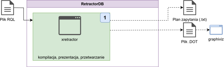
Fig. 26. The compilation process
As an example file for compilation, we’ll use a file query.rql with the following content:
DECLARE a INTEGER STREAM core0, 0.1 BINFILE 'datafile1.dat'

SELECT str1[0]+1 STREAM str1 FROM core0>2
This is a very simple example of a file containing two directives. The first declares the existence of an ephemeris in the form of a binary data source containing 4-byte INTEGER values. Data from this file will be read at a rate of 10 times per second. And the name of this object is core0.
The second command creates an artifact named str1, taking ephemeral data shifted in time by two reads, i.e. 0.2 seconds. While building successive elements of the output stream, the data read from core0 is processed, and the value 1 is added to every value read.
To compile this file, the following command must be invoked:
$ xretractor -c query.rql
The following system response will be printed on the screen:
core0(1/10)	datafile1.dat
	a: INTEGER
str1(1/10)	origin=2
	:- PUSH_STREAM(core0)
	:- STREAM_TIMEMOVE(2)
	str1_0: INTEGER
		PUSH_ID(str1[0])
		PUSH_VAL(1)
		ADD
Omitting the -c parameter will cause the system to attempt compilation and immediately send the compiled query execution plan for execution. This will cause an error, since the data file datafile1.dat presumably hasn’t been prepared yet.
Besides the text view, we can also look at the compilation output in graphical form. To do this, invoke the following sequence of commands:
$ xretractor -c -d -f -t -s query.rql > out.dot && dot -Tsvg out.dot -o out.svg
Assuming you have the dot program from the graphviz package installed in your runtime environment, this command will generate an image file showing the system’s response in the form of a graph.
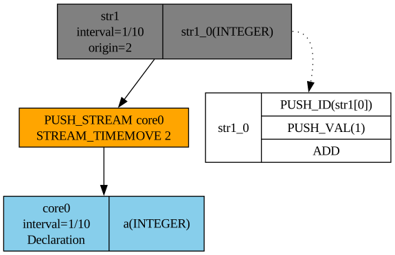
Fig. 27. Graphical representation of a query plan
RetractorDB can generate an image in response to one of the requested data-processing chains. The graphical presentation is most suitable for creating and presenting data-processing graphs. Unfortunately, readability suffers for very complex schemas.
Fig. 27 shows the trivial query execution plan produced by compiling the two-line query.rql file. At the very top we see the object str1, producing artifacts at a rate of 10 records per second. Information about the artifact-creation rate does not appear in the query; it is computed based on the algebraic expression in the FROM clause of the SELECT query. We can also see how successive records of the str1 stream are produced. Here we have a typical stack-based data-processing algorithm. First, the ephemeral value produced by the algebraic expression is pushed onto the stack, then the value 1 is placed on the stack. The ADD instruction pops both values off the stack, leaving the sum on the stack. What remains on the stack - i.e. the result of the addition - is placed into the field of the record being created.
On the other side we see stream operations. Stream operations are carried out in a different domain. There, we process objects of one or two values. Operations act either on two streams, or on a single stream with an argument. The classic stack has no application for algebraic stream operations. For simplicity, the notation resembles stack operations somewhat. We see, in the attached example, that operations on current data are carried out by shifting the data in time by 2. I deliberately do not say that this is 2 seconds - here 2 denotes a relative value with respect to the arrival rate. For an arrival rate of 10 samples per second, the value 2 means a time shift of 0.2 seconds.
Complex algebraic expressions involving at least two stream operators give rise to the substrates mentioned in previous chapters. Every query whose FROM-clause algebraic expression contains more than one operator is broken down into interdependent two-argument operations. The substrate’s argument list is, by default, the full expansion of the schema.
Available xretractor flags
Different sets of flags are available in compile mode (-c) and in execution mode. Below are the compile-mode flags used for generating graphs:
| Flag | Full name | Meaning |
|---|---|---|
-c | --onlycompile | compile only - does not start processing |
-d | --dot | generate output in DOT (graphviz) format |
-f | --fields | show stream fields in the DOT graph |
-t | --tags | show individual field programs (requires -f) |
-s | --streamprogs | show stream programs in the DOT graph |
-u | --rules | show RULE rules in the DOT graph |
-p | --transparent | transparent background for the DOT graph |
-i | --hideruleprog | hide the rule-condition program (with -u) |
-m | --csv | output in CSV format |
Execution-mode flags (without -c):
| Flag | Full name | Meaning |
|---|---|---|
-m N | --llimitqry N | run N processing cycles, then exit |
-k | --noanykey | don’t wait for a keypress - daemon/script mode |
-t | --realtime | real-time mode (SCHED_FIFO, mlockall) |
-x | --xqrywait | wait until the first xqry command has been handled before starting |
-s | --status | check whether an xretractor instance is already running |
-v | --verbose | print stream parameters at startup |
-j | --service | service mode - log to stderr (journald) |
-g F | --config F | TOML configuration file instead of the search order |
-b | --build-info | print the optimizer configuration and exit |
ℹ️ Info
The
-m Nparameter counts iterations of the main loop, not seconds. For streams with a 0.1 s interval (10 Hz),-m 10means ~1 second of processing.
⚠️ Warning
When receiving the results of a run limited by
-m Nthroughxqry, add-x(--xqrywait). Without this flag, the server may process the entire budget before the client connects. The gate is released after the first command has been handled:xqry --selectregisters its subscription before computation starts. Another client’s--diror--helloalso releases the gate, so it is not a readiness barrier for all receivers. When inspecting artifacts after the process has finished,-xis not needed and will hold up the run if no client command arrives.
A full list of all options with a description of each - including the --realtime option, which requires system privileges - can be found in Appendix A.
Data Processing and Distribution
Starting the data-processing process and analyzing the diagram shown in Fig. 14, we can identify the following flow - Fig. 28:

Fig. 28. Control-flow diagram of the processing workflow
To carry out the processing, we’ll need to prepare data and build a data-processing chain. As input to this chain we’ll use a prepared query-plan file, and we’ll prepare a binary file with data. We’ll build a process that processes the data and displays the results.
We’ll change the source query.rql file to the following:
DECLARE a INTEGER STREAM core0, 0.1 TEXTFILE 'datafile1.txt'
DECLARE a BYTE STREAM core1, 0.2 DEVICE '/dev/urandom'

SELECT str1[0], str1[0] + str1[1]/20 STREAM str1 FROM core0 + core1
In this example we declare the existence of a text file containing text data. I suggest filling the file datafile1.txt with the following content:
$ seq 20 28 > datafile1.txt
20
21
22
23
24
25
26
27
28
The file will contain consecutive numbers from 20 to 28.
A look at the query execution plan gives us the picture in Fig. 29:
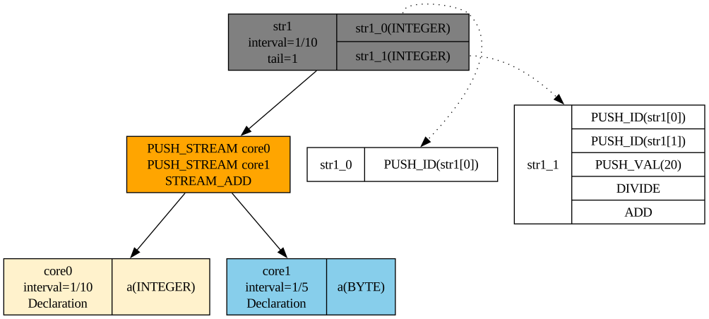
Fig. 29. Graphical representation of query plan 2
Once we’ve prepared the data file, we can start the compilation and data-processing process. We do this by running the following command:
$ xretractor query.rql
And here an important property of the system comes into play. The system should immediately begin executing the process. Any key pressed in the terminal will interrupt this process.
I suggest opening a second terminal window and continuing the session there. In the second terminal window we can run the following command:
$ xqry -d
name  | duration | size | count | location      | cap
------+----------+------+-------+---------------+----
str1  | 1/10     | 6912 | 864   |               | 0
core0 | 1/10     | -1   | 49    | datafile1.txt | 1
core1 | 1/5      | -1   | 25    | /dev/urandom  | 1
Something similar should appear. Of course, the counters for str1 should differ. It’s logical that with every read we’ll get larger values for the accumulated size of the str1 stream.
If we want to see, on screen, what’s happening inside the data-processing process right now, I suggest issuing the command below, and after a few lines appear on screen, pressing any key to interrupt the process:
$ xqry -s str1
20 26
21 33
22 34
23 27
24 28
25 35
26 36
27 28
The first column contains the sequence of numbers - exactly as we entered them into the datafile1.txt file. The second column contains the result of processing. A value taken from the pseudo-random number generator, divided by 20, is added - the second column flows along beneath the first.
How can we see this graphically? I suggest running the following command:
$ xqry -s str1 -p 50,50 | gnuplot
The following window will appear on screen, with data streaming in live:
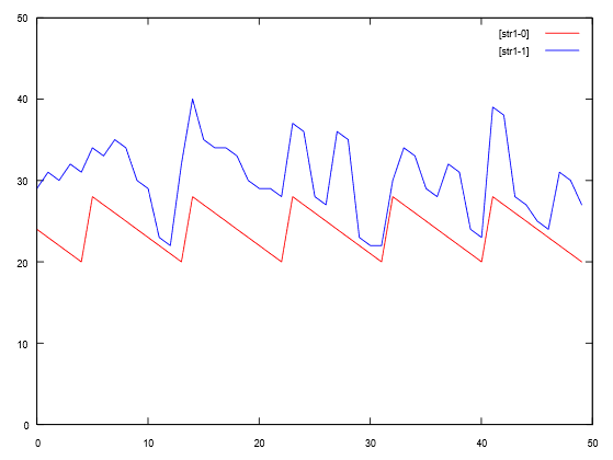
Fig. 30. Snapshot of the gnuplot window showing incoming data
In Fig. 30 we see what the data represented numerically looks like. The sawtooth shape is the first column; the irregular shape wrapping around the sawtooth is the second column. The figure shows a static snapshot - but in the actual window, this data streams in and the picture updates continuously.
A typical way to send data outside the machine on which xretractor and xqry are running is to use the command:
$ xqry -s str1 | nc -l 8888
on the second computer, you need to write:
$ nc server_name_or_ip 8888
ℹ️ Info
The
-pflag in netcat (BSD syntax) is not supported by the GNU netcat available on modern Ubuntu/Debian systems. The correct syntax isnc -l 8888(without-p).
Data transmission will take place over the network.
If we want to stop the xretractor process using the xqry command, we can run the following command:
$ xqry -k
After issuing this command, the xretractor process will shut down and interrupt the query plans being processed.
A recording of the process shown on screen (Fig. 31) looks as follows:
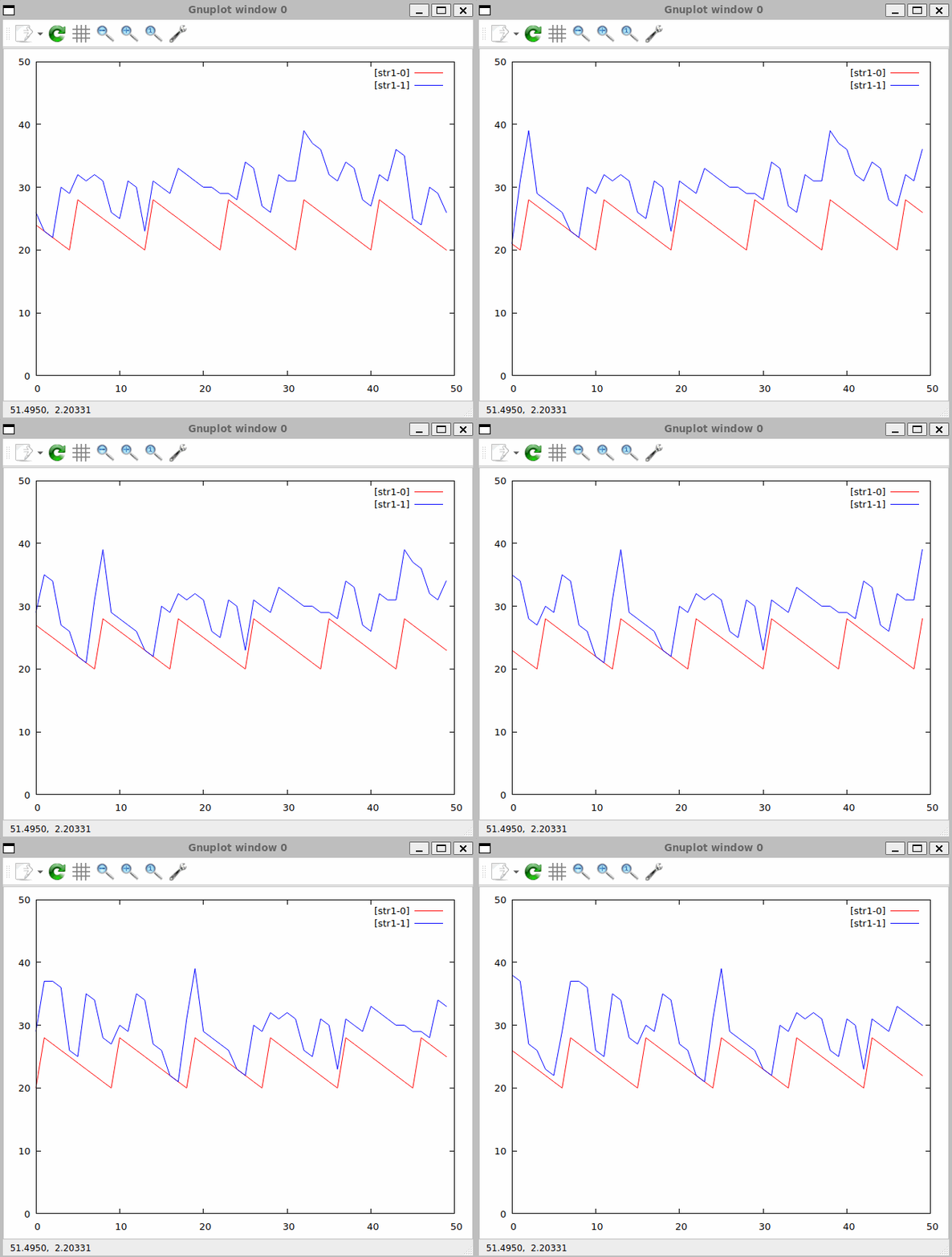
Fig. 31. Recording of real-time data processing
Artifact Analysis
Looking more broadly at the potential data paths in Fig. 14, the last undescribed path is the one involving the xtrdb tool.
While building the system, I needed a tool for accessing artifacts in order to run integration tests. To verify correctness, I had to compare processing results at various stages. Fig. 32 shows the complete data flow, including the role of the xtrdb tool.

Fig. 32. Data flow in artifact analysis
To present the artifact-analysis process, the entire processing chain needs to be taken into account. We’ll use the same query as before. However, we’ll run our data-processing process a bit differently this time.
$ xretractor -m 10 query.rql
A query-processing run invoked this way will finish after 10 processing cycles. The -m parameter specifies the number of iterations of the main loop, not the number of seconds - the running time depends on the interval of the source streams. For streams with a 0.1 s interval (10 Hz), this means ~1 second of runtime. After it finishes, and we look at the directory in which we ran the query, we should see the following files:
$ ls -al
total 32
drwxr-xr-x  2 michal michal 4096 Oct  4 18:01 .
drwxr-xr-x 10 michal michal 4096 Oct  4 17:59 ..
-rw-r--r--  1 michal michal   51 Oct  4 18:01 core0.desc
-rw-r--r--  1 michal michal   43 Oct  4 18:01 core1.desc
-rw-r--r--  1 michal michal   27 Oct  4 17:59 datafile1.txt
-rw-r--r--  1 michal michal  180 Oct  4 18:00 query.rql
-rw-r--r--  1 michal michal   72 Oct  4 18:01 str1
-rw-r--r--  1 michal michal   34 Oct  4 18:01 str1.desc
As you can see, three .desc files were created, plus one file containing artifacts. If we look inside the str1 file, we’ll see fairly modest content:
$ hexdump str1
0000000 0014 0000 0015 0000 0015 0000 0016 0000
0000010 0016 0000 0017 0000 0017 0000 0018 0000
0000020 0018 0000 0019 0000 0019 0000 001a 0000
0000030 001a 0000 001b 0000 001b 0000 001c 0000
0000040 001c 0000 001d 0000
0000048
Alongside the artifact file, metadata files are also created. Their content describes the structure of the file.
$ cat str1.desc
{       INTEGER str1_0
        INTEGER str1_1
}
The descriptions of the ephemeris files are far more interesting. The description files for ephemeral data point to files in the Linux filesystem.
$ cat core0.desc
{       INTEGER a
        REF "datafile1.txt"
        TYPE TEXTSOURCE
}
$ cat core1.desc
{       BYTE a
        REF "/dev/urandom"
        TYPE DEVICE
}
Metadata description files are created automatically the moment an object is registered in RetractorDB. Remember to delete these descriptors if you modify the query.rql file.
Once the xtrdb program is started in a terminal, the tool displays a dot (.) as its prompt. This character is just a prompt - it is not part of the command. You can start interacting with the tool right away. Example session:
$ xtrdb
.open str1
ok
.desc
{       INTEGER str1_0
        INTEGER str1_1
}
.list 1
{ str1_0:20 str1_1:21 }
.quit
Working with this tool feels like working with a classic, old-school dbase database. There’s no state machine here, no loops or conditions - just reading and modifying binary files described by metadata.
The main goal of this tool was to support the creation of test scripts. RetractorDB is deterministic. The system has no race conditions - data that arrives on the input should always produce the same results on the output. Unless, of course, we mix in random data, as in the example shown here.
NOTE: The functionality described here is covered by the tests:
issue113_meta_xtrdb,issue113_meta,issue113_null_txtsrc,Pattern5, described in the appendix Integration Tests.
A very useful feature of this tool is the list and rlist functions - listing the initial elements of a file, or the final elements of a file, respecting the structure described in the metadata.
.list 4
{ str1_0:20 str1_1:21 }
{ str1_0:21 str1_1:22 }
{ str1_0:22 str1_1:23 }
{ str1_0:23 str1_1:24 }
.rlist 4
{ str1_0:28 str1_1:29 }
{ str1_0:27 str1_1:28 }
{ str1_0:26 str1_1:27 }
{ str1_0:25 str1_1:26 }
I encourage you to experiment and browse the source of this tool. It’s one of the less complicated, yet very useful, parts of RetractorDB.
Inspecting null/gap metadata
Every artifact has an associated .meta index file, described in detail in the chapter on the storage format. Its content can be viewed directly in xtrdb with the meta command:
.open str1
ok
.meta
record 0: count=9 gap=false nullBitset=00
The gap=false entry means there is no gap in the data; nullBitset shows which fields contain null values (one bit per field). Data with no gaps at all forms a single entry count=N, where N is the total number of records.
Summary
In summarizing, it’s worth pointing out the scope of knowledge this chapter conveys. Here I wanted to show how the individual parts of the system can be run, and what the command sequences look like on which we build further functionality using RetractorDB.
I tried to reduce the number of potential commands to a minimum. At present I have effectively reduced the set to 3 commands. I believe a system designed this way will be maximally useful and reasonably efficient. Complexity is a separate matter. Explaining the processing itself - the new algebra, and why a plus sign doesn’t mean plus - is, in itself, difficult. I hope, though, that once a certain barrier of understanding is crossed, the rest becomes obvious. The decisions made were the result of reflection, trial, and error. I want to emphasize that, quite simply, I did not find a better method.
Query Compilation
An attentive reader will probably notice that, in the compiled query execution plans shown in the previous chapter, certain values don’t match what was written in the query.
The compiler, while building a query plan, carries out the process autonomously. Sometimes it feels like you ask for one thing and get something else - at first glance this behavior seems entirely counterintuitive. And as a user, I fundamentally have no control over it. Interestingly, the outcome of the query does correspond to what I asked for in the query. Perhaps the correct title for this chapter should be: Why does the compiler do things its own way, and claim to know better?
In this chapter I want to explain how I solved the syntactic problems I encountered while building the query language.
Compiler input and output
The .rql file
Compiler input - text in the RQL language containing DECLARE, SELECT, and RULE statements as well as configuration directives (e.g. :STORAGE). The ANTLR4 parser reads the file statement by statement.
The order of DECLARE and SELECT in the file does not matter: a query may refer to a stream defined further down, because dependencies between streams are resolved only by the compiler. RULE is the exception - the parser attaches a rule to a stream that has already been read, so a rule must come after the definition of its stream; otherwise the parser reports Rule '…' refers to stream '…', but no such stream is defined. A reference to a stream that does not exist anywhere in the file stops compilation with Referenced Stream in QUERY _not found_ in CORE TREE.
The ANTLR4 parser → qTree
The parser builds the internal representation qTree - a std::vector<query> - by appending one element for every DECLARE and SELECT statement and configuration directive, in file order and without sorting. A SELECT element carries the field schema with its stack programs and the FROM program that names the source streams. At this point the time interval (delta) is known only for DECLARE declarations; for SELECT queries the compiler determines it. A STREAM name[N] generator template is still a single element, and a RULE does not create an element of its own - it goes onto the rule list of its stream.
The order of the vector changes during compilation: interval resolution sorts it by delta, and the topological order (producer before consumer) is restored only by the last stage.
The 23 compilation stages
qTree passes through an ordered chain of transformations: from breaking down FROM expressions into two-argument operations, through determining deltas, simplifying expressions, and locating fields, all the way to semantic verification, buffer-size computation, and the final topological sort. Each stage assumes the previous one succeeded.
Execution plan → dataModel
At the output of compilation, every query in qTree has: a field schema with types and offsets, a delta, buffer sizes, and a ready instruction sequence. dataModel takes over this plan and executes it cyclically in real time.
The -c flag stops xretractor after this step and prints the plan to standard output - without starting processing.
Overview of topics covered in this chapter
The chapter is structured following the order of the compiler’s stages - from a description of the data structure and the chain of stages, through the individual transformations, to error handling.
-
Describes the entire chain of stages in the
compiler::compile()function. Compilation is not a single step - it is an ordered sequence of twenty-three stages over the internalqTreerepresentation, from expanding generators and reducing FROM expressions to two-argument form, through determining intervals, validating substrate names, simplifying expressions, and locating fields, all the way to semantic verification, buffer allocation, and the final topological sort. Each stage assumes the previous one succeeded, and an error at any stage stops compilation. -
Describes the DAG structure produced during compilation - the foundation on which every stage rests. The roots are ephemeris declarations (external sources); inside the graph lie intermediate substrates; and the leaves are artifacts. The
-dflag generates output in DOT format, whichgraphvizturns into a visual dependency graph. The order ofDECLAREandSELECTin the.rqlfile does not matter - the compiler builds the dependency graph; only aRULEmust come after the definition of the stream it refers to. -
Explains the
extractIntermediateStreamsstage - the first step after generator expansion. When a FROM expression contains more than two arguments (e.g.(core0#core1)+core2,core0+core1+core2), the compiler breaks it down into two-argument operations and creates named substrates. A later stage,deduplicateSubstrats, detects when a substrate is structurally identical to a user query and replaces the references - avoiding duplicate computation. -
Explains the
expandSchemaWildcardsstage. The*symbol in a SELECT clause is replaced with the full field list derived from the source stream’s schema - including fields arising from stream-sum operations. An example shows how field types determine which field ends up in which position of the resulting schema. -
Describes the
resolveStreamIntervalsstage. The compiler determines the delta of every output stream from the stream-algebra equations: for the+operator the delta is the minimum of the inputs, for#it’s the harmonic mean, for@(step, window)it’s a derivative of the window size. The algorithm runs iteratively - each round resolves at least one stream, until all deltas are known. -
Describes the mechanism built into the
resolveStreamIntervalsstage. If the number of unresolved streams stops decreasing, no stream can obtain a delta - a sign that the dependency graph contains a cycle. Compilation ends with the error"Circular dependency in stream definitions". The chapter includes an example of a cyclic query and how to fix it. -
Describes the
resolveFieldReferencesandlocalizeFieldOffsetsstages. After a sum+, an output field can be referenced either by its index in the combined schema (str1[1]) or by the source stream name with a local index (core1[0]). After an interleave#, the components share one schema, so named references to components are rejected; use the output stream name or de-interleave with&/%. -
Describes the
expandIndexWildcardsstage - syntactic sugar for parallel operations on pairs of fields. The_symbol in an index causes the formula to be repeated for all compatible slots that the referenced stream contributes to the record produced by the completeFROMclause. Thussrc[_] * coef[_]withFROM src@(1,5)+coefgenerates five products even thoughsrcitself has only one field. Use case: building signal-filter queries. -
Defines the type-promotion rules that apply throughout the compilation chain. The result of
BYTE * INTEGERhas typeINTEGER- the compiler determines the output field’s type statically, before any data is processed. The complete type hierarchy supported by RetractorDB is also described. -
Gathers diagnostic tools in one place: the
-cflag for plan inspection, the-c -d -f -spipeline for graph visualization viagraphviz, a table of plan-instruction meanings (PUSH_ID, PUSH_STREAM, STREAM_ADD, …), and a catalog of common compilation errors with their causes and fixes.
Compilation Passes
Query compilation in RetractorDB proceeds through multiple stages. Each stage transforms the internal representation of the queries - the qTree tree - and passes the result to the next one. The order is strictly fixed: every stage assumes the previous one succeeded.
qTree is a std::vector<query> - the central data structure of the compiler and executor. Every element corresponds to one query (SELECT or DECLARE) and stores its field schema, stack-instruction sequence, time interval, startup tail, and references to source streams. Not every stage preserves vector order: interval resolution sorts it by rInterval. Compilation therefore ends with an unconditional topological sort, which guarantees that a producer precedes its consumer during execution.
Running example
Throughout the chapter we follow a single query - query.rql - through the successive stages:
DECLARE a BYTE, b INTEGER STREAM core0, 0.1 TEXTFILE 'sensor_a.txt'
DECLARE c INTEGER, d FLOAT STREAM core1, 0.2 TEXTFILE 'sensor_b.txt'
DECLARE e INTEGER STREAM core2, 0.3 TEXTFILE 'sensor_c.txt'

SELECT *                    STREAM merged FROM core0 + core1
SELECT merged[0], merged[2] STREAM result FROM merged
After passing through all the stages, xretractor -c query.rql prints:
core0(1/10)	sensor_a.txt
	a: BYTE
	b: INTEGER
core1(1/5)	sensor_b.txt
	c: INTEGER
	d: FLOAT
merged(1/10)	tail=1
	:- PUSH_STREAM(core0)
	:- PUSH_STREAM(core1)
	:- STREAM_ADD
	core0_0: BYTE
		PUSH_ID(merged[0])
	core0_1: INTEGER
		PUSH_ID(merged[1])
	core1_2: INTEGER
		PUSH_ID(merged[2])
	core1_3: FLOAT
		PUSH_ID(merged[3])
result(1/10)	tail=1
	:- PUSH_STREAM(merged)
	result_0: BYTE
		PUSH_ID(result[0])
	result_1: INTEGER
		PUSH_ID(result[2])
core2(3/10)	sensor_c.txt
	e: INTEGER
The plan is printed in the final topological order: the declarations core0 and core1 precede their consumer merged, which precedes the query result. The unused declaration core2 goes last. tail=1 is the startup tail determined by computeStartupLatency. PUSH_ID references point to positions in the query’s input record, written under the query’s own name: result[2] is the third field of the merged record, that is core1.c.
The field list of result refers only to the stream in its own FROM clause. Writing core1[0] there ends in the compilation error Stream 'result' refers to 'core1', which is not in its FROM clause: core1 is a source of merged, not of result - see Aliasing.
The subchapters on substrates and the _ symbol use extended variants of the same set of declarations. For how to interpret every element of this plan, see Compilation Debugging.
The chain of stages
The chain of twenty-five stages is defined by the compiler::compile() function:
checkFunctionCalls- scalar-function names and aritycheckStreamReducerFieldRefs- stream reducer outside theFROMclauseexpandStreamGenerators- expansion ofname[N]stream familiessnapshotNamedSourceRefs- snapshot of user-written referencesextractIntermediateStreams- two-argumentFROMexpressions, substratesexpandSchemaWildcards- expansion of*and[_]resolveStreamIntervals- stream intervals, loop detectionfactorMatchedHashTimeMoves- factoring a common shift out of an interleavededuplicateSubstrats- elimination of repeated substratesvalidateSubstratNameUniqueness- unambiguous substrate namesresolveFieldReferences- field references as flat indexesresolveWindowAggregates- record-history aggregate groupsinferFieldShapes- type, length, and cardinality of every fieldcheckRuleConditionShapes- computability ofRULEconditionssimplifyFieldExpressions- simplification of field and rule programsshareEquivalentSelectComputations- sharing equivalentSELECTcomputationslocalizeFieldOffsets- field offsets in the input buffercomputeLogicalOrigin- logical origin of a streamcomputeStartupLatency- startup tailcomputeRequiredCapacities- required buffer historyvalidateConstraints- semantic validation of the planapplyCapacitiesToStreams- capacity applicationcheckHistoryMemory- RAM history budgetapplyDiskRetention- default file retention and available historytopologicalSort- final producer–consumer order
The stages factorMatchedHashTimeMoves, deduplicateSubstrats, simplifyFieldExpressions, and shareEquivalentSelectComputations are optimizations that the RDB_OPT_* switches can disable. Disabling them does not change result values; at most it can lengthen the startup tail (see factorMatchedHashTimeMoves). All other stages always run.
checkFunctionCalls
Validates scalar-function names and arity against the single rqlFunctions.hpp table. Matching is case-insensitive and the canonical spelling is stored in the token. An unknown function or invalid width stops compilation through Check result: before generator expansion, so one template error is not multiplied N times.
checkStreamReducerFieldRefs
Rejects a stream reducer (MIN, MAX, AVG, SUMC without a window width) used in a SELECT field program or in a RULE condition. The grammar admits it in a scalar expression, but no execution mechanism evaluates it there: the query SELECT avg STREAM o FROM AVG(src) used to pass compilation and then never emitted a single record. A stream reducer belongs in the FROM clause; the working SELECT * FROM AVG(src) is not affected by this check. The stage sits next to checkFunctionCalls for the same reason - before generator expansion.
expandStreamGenerators
Expands every SELECT ... STREAM name[N] ... template into N ordinary queries named name$0…name$(N-1) and substitutes the instance ordinal for $ in fields, values, and FROM references. It is the first pass that rewrites the plan (only the checkFunctionCalls and checkStreamReducerFieldRefs checks precede it): everything after it receives a plan indistinguishable from hand-written queries. See SELECT Command for syntax and constraints.
Before copying a template it also checks the number of streams after expansion: at most 148. See Plan Size Limits for the other bounds.
snapshotNamedSourceRefs
Snapshots source references written by the user before substrates are created. Later field localization uses the snapshot to distinguish legal synthetic tokens from references to a component of #, whose identity is no longer preserved by the result.
extractIntermediateStreams
Reduces every FROM expression to at most a two-argument form. Complex expressions like (core0#core1)+core2, and chained notations without parentheses (core0+core1+core2, core0#core1#core2), require intermediate streams. Every query is reduced to a fixed point, so the stage also handles adjacent unary subexpressions such as (core0>2)#(core1>1). This stage automatically creates substrates - see Substrates.
expandSchemaWildcards
Expands both * in the SELECT clause and the [_] index. It replaces an asterisk with fields derived from the source schema. A formula containing x[_] is replicated according to the number of slots that x contributes to the record produced by the complete FROM clause, rather than the width of stream x itself. A one-field x under the window x@(1,5) therefore yields five elements. If the named contribution does not form a contiguous block of fields in FROM, compilation fails instead of assuming an arbitrary width.
At this stage, derived schemas expand a numeric T[N] entry into N scalar fields. A declaration descriptor still retains one array entry, while byte layout and flat-slot order remain unchanged. STRING[N] remains one text field. Stream operators, reducers, AGSE, and payloads therefore use the same indexing unit. See Asterisk Expansion and Underscore Symbol Processing.
resolveStreamIntervals (← loops are detected here)
Determines the time interval (delta) of every stream based on the algebraic operators and the intervals of the input streams. An iterative algorithm resolves as many streams as possible in each round. A record-history aggregate in the SELECT list does not change the interval and requires one plain stream reference in FROM; a compound clause is rejected here. The pass detects cyclic dependencies by stopping when the number of unresolved streams stops decreasing - see Interval Resolution and Loop Detection.
factorMatchedHashTimeMoves
Recognizes matched shifts of interleave arguments. When i·ΔA=k·ΔB, it rewrites (A>i)#(B>k) as (A#B)>(i+k), reducing two shift substrates to one interleave substrate. Unmatched cases and substrates shared with other consumers remain unchanged - see Substrates.
A shift moves silence into the logical origin rather than inserting prefix records. Equality of the physical shifts makes both sides of the rule carry the same emitted sequence and the same logical origin. The tails are not equal: the factored side reads content directly from the interleave, so it is ready no later - and usually earlier - than the side that reads components after their own shift. The rule is therefore a latency optimization, not a neutral rewrite; for the scope of theorem R1 and a counterexample see Formal foundations and proofs.
deduplicateSubstrats
An optimization: if two queries use the same intermediate operation (e.g. core0#core1), this stage points the second query at the substrate created by the first. It avoids duplicate computation - see the example in Substrates.
validateSubstratNameUniqueness
Checks that two substrates with the same name denote the same program. Names longer than 200 bytes are shortened deterministically by composeStreamName(), so this check turns an extremely unlikely 64-bit digest collision into a loud error instead of an ambiguous plan. It runs independently of optimizer switches and after deduplication, because identical duplicate names are a normal transient state before that point.
resolveFieldReferences
Turns references to fields from source schemas into flat indices in the output schema. It handles aliases after sum - turning core0[0] into str1[0], for example - and records the source to which a bare field name was resolved. Named references written by the user are tracked separately so a later pass does not confuse them with tokens synthesized by the compiler. A bare numeric-array name is rejected: a does not mean a[0]; an element must be selected. See Aliasing.
resolveWindowAggregates
Extracts the argument program of each window aggregate - MIN, MAX, AVG or SUMC(expression : W) - in the SELECT list into query::windowGroups. It validates positive width, numeric type, one history source, at least one field read, and the bans on nesting and RULE use. Identical source–expression–width triples share a group and one history scan. The aggregate token becomes a zero-argument operand that points to the computed group result.
inferFieldShapes
The only stage that establishes the public shape of a SELECT field: its type, length, and cardinality. The shape follows from the whole field program - the pass replays the runtime arithmetic on a stack of types, including BYTE promotion, explicit conversions in the middle of an expression, the result of a record-history aggregate, and the width of STRING. The stage replaced the earlier local rules (propagateCopiedFieldShapes, inferStringFieldTypes), which settled the shape only in selected cases - see Type Promotion.
The pass runs to a fixed point because the tree is still sorted by interval and a consumer may precede its producer. It covers only nodes that copy their operand’s schema; reducers and the @ window keep the schema built by their operator, and DECLARE declarations are left untouched. The stage precedes expression simplification: after constant folding, a field’s width would depend on an optimization switch.
checkRuleConditionShapes
Applies to RULE conditions the same computability check that inferFieldShapes applies to fields. A rule condition is executed by the same expression evaluator, so without this stage an invalid condition would bypass the check and silently produce a wrong value. The pass writes nothing into the plan - it only rejects conditions that cannot be computed.
simplifyFieldExpressions
Simplifies SELECT field programs, record-history aggregate arguments, and RULE conditions after references have been resolved but before equivalent computations are shared. The pass folds constant expressions, combines safe constant tails in integer arithmetic and STRING concatenation, and removes type-compatible neutral elements (E+0, E-0, E*1, E/1). With the separate aggressive_expr_optimization=ON switch it writes a repeated exact factor as a power, for example E*E*E as E^3; this rule is disabled by default.
The pass preserves NULL semantics and type promotion. It therefore does not simplify E*0, reassociate FLOAT or DOUBLE operations, or alter programs whose type or operation cannot be established safely. Repeated-factor folding is limited to types with exact multiplication (BYTE, INTEGER, UINT, and RATIONAL); it does not replace one FLOAT or DOUBLE multiplication with a call to pow.
Constant-tail reassociation (rule B) requires exact value equality, including NULL, with optimization enabled or disabled. For an INTEGER, UINT, or BYTE base and INTEGER constants, the guard computes the intervals of base values for which the intermediate result and the rewritten result fit their representation. A rewrite is allowed only when the rewritten result’s defined domain is contained in the intermediate result’s defined domain. For BYTE the guard uses the complete INTEGER range because a compound base, such as b+b, already produces INTEGER. It therefore retains the sequential forms of (i+1)-1 at INT_MAX, i*-1*-1 at INT_MIN, and u*-2*-3 and u+5-3 over UINT, preserving intermediate overflow as NULL.
Rule B refuses reassociation for RATIONAL and other unproved promotions; constant folding and removal of type-compatible neutral elements remain available. STRING concatenation remains allowed. The it_expr_corpus-value regression covers INTEGER/UINT boundaries, BYTE promotion, RATIONAL overflow, and the u+3-5 control; it checks values and descriptors under all-off as well.
shareEquivalentSelectComputations
Detects explicit SELECT queries with equivalent field programs and FROM trees containing STREAM_ADD. It orders only the two children of an individual STREAM_ADD node without changing the grouping of the complete tree. For each equivalence class it creates one STREAM_SELECT_* substrate and retains the public queries as lightweight projections with their own names, descriptors, rules, and storage. The pass runs before field-offset localization - see Substrates.
localizeFieldOffsets
Converts field references (b[x], c[y]) into positions in the query’s flattened input record, written under the query’s own name (result[z]). For sum +, the offset follows from the number of fields in the preceding components. For interleave #, both arguments share the same positions in one schema; component identity is no longer available through its name.
A position can be determined only for streams in the FROM clause and for sources reached through compiler-generated substrates. A reference to a source of an intermediate stream that is a user query - e.g. core1[0] with FROM merged - stops compilation with Stream '…' refers to '…', which is not in its FROM clause. Such a stream has its own interval and buffer, so the position of its sources in the consumer’s input record cannot be determined.
At this stage the compiler rejects user-written A[0], A.field, A[_], A.*, and bare field names if they refer to a component reached through #. The check also covers RULE conditions and sources hidden behind automatic substrates. References through the output stream name, an unqualified *, and explicit component recovery with & or % remain legal.
computeLogicalOrigin
Computes query::logicalOrigin, the index of the first record that exists at all. The difference from the tail is qualitative: the tail says “not yet”, the origin says “this record has no definition”. The origin originates from the @(k,L) window stamped by the interval end - its early records would reach before the start of the source - from a history aggregate, which adds W-1, and from the shift >N, whose record n carries record n-N. Every other operator merely propagates the origin, through the same index mapping it reads with.
For @ and >N the form is closed; for +, #, -, Theta and ~Theta the pass searches for the smallest index reaching the component threshold, by bisection over a non-decreasing mapping. The plan listing shows origin=.
computeStartupLatency
Computes query::startupLatency, the number of initial slots of the stream’s own interval in which an existing result is not yet ready. Sources have tail 0; >N gives max(0, W_src − N), because it reads a record older than the current one; interleave includes both input tails and its own look-ahead on the second argument; sum takes the maximum of both inputs’ availability bounds. Difference and both de-interleaves use exact phase bounds - left de-interleave does not unconditionally add one slot. AGSE uses the bound from the newest field in its window, and reductions and record-history aggregates add no own tail. The plan listing shows tail= and the runtime emits no record during the tail. The number of silent slots is origin + tail.
This pass runs after computeLogicalOrigin and before capacity computation: the tail depends on which slots are records, and retained history depends on the consumer’s first emission time.
computeRequiredCapacities
Computes required buffer capacities from the distance between the producer’s head and the index read by a consumer. For a >N shift, the backward distance is W_out-W_src+N, so the base capacity is W_out-W_src+N+1. If the source is a declaration, two look-ahead records are added: the record armed when storage is opened and the zero prefetch. The result is clamped to at least one record. History capacity is an execution requirement, not a result prefix.
A record-history aggregate requires at least W consecutive records of its named source. Capacity also accounts for logical origin, tail, and interval differences like every other history read; it is not selected as a local W alone.
validateConstraints
Verifies semantic correctness of the compiled plan: type and flat-width compatibility, window sizes, source availability, and operator constraints. Interleave # requires equal flat schemas whether an input was written as T[N] or as N scalar fields.
applyCapacitiesToStreams
Applies the computed capacities to the stream objects. A MEMORY store keeps the greater of RETENTION n and the plan’s need; declared sources take their capacity from consumer needs.
For an interleave, the compiler reduces \(\Delta_a/\Delta_b=p/q\) to coprime positive \(p,q\) and scans one full phase period \(p+q\). For each slot \(i\) of that period it determines which component the interleave selects and at which index \(j(i)\), then takes the maximum of the required latency:
\[ W_{\#} =\max_{0\le i<p+q}\left( \left\lceil\frac{\bigl(j(i)+1+W_{s(i)}\bigr)\Delta_{s(i)}}{\Delta_c}\right\rceil -1-i \right) \]
The scan result is exact - it neither undershoots nor overshoots the causal bound. The arithmetic runs in 64 bits, because the product \((j+1+W)\cdot\text{numerator}\cdot\text{denominator}\) exceeds int range even for moderate intervals. Above kHashPhaseScanLimit, HashStartupLatency() (SOperations.hpp) uses a safe bound without a phase scan:
\[ W_{\#,\mathrm{fallback}} =\max\left( \left\lceil\frac{W_a\Delta_a}{\Delta_c}\right\rceil, \left\lceil\frac{W_b\Delta_b}{\Delta_c}\right\rceil +\left\lceil\frac{p+q-1}{p}\right\rceil \right) \]
The first two terms convert the input tails into output slots; a zero tail contributes zero. The term \(\lceil(p+q-1)/p\rceil\) describes only the phase and is insufficient on its own for nonzero input tails. The complete bound is conservative: it does not release a record before its dependencies are ready, but it does not promise an excess of exactly one slot. The regression ut_soperations::xSOperations.hash_startup_latency_above_scan_limit_stays_safe compares it with an independent scan, including nonzero input tails.
Regressions cover ratios including \(3/5\), \(3/2\), \(7/11\), and \(160/147\), including periodic all-NULL records in the blocked, non-rewritten left-hand side of the R1 identity; the operator formula itself is guarded by ut_h10aGate.
checkHistoryMemory
Sums the history cost of DECLARE sources and MEMORY rings after their capacities are fixed. If it exceeds [limits] history_memory_mib, it returns an error with the byte count and the stream with the largest share. File stores are excluded.
applyDiskRetention
Applies [storage] default_retention to DEFAULT and DIRECT streams without explicit retention, including substrates. For a bounded segment count, it checks that the plan’s required history fits the shortest state just after rotation: (segments - 1) * capacity + 1 records. Otherwise compilation fails with the stream, retention, and required depth. segments = 0 means unbounded history and is exempt from this check.
topologicalSort
Unconditionally restores final producer–consumer order. This is part of execution correctness, not presentation: a # result has a smaller interval than its inputs, so earlier interval sorting can place the consumer before its producers.
Plan-rewriting passes are additionally wrapped in verifyUserFieldNamesPreserved(). Optimization may change or remove internal substrates, but it cannot change field names of a public stream, because those names enter the observable .desc descriptor.
Check and rewrite stages return "OK" or an error message - in which case compilation stops. snapshotNamedSourceRefs, computeRequiredCapacities (which returns the capacity map), and topologicalSort return no result of this kind. Some plan inconsistencies, such as a reference to a nonexistent stream, stop compilation with an exception instead of a message.
Plan Size Limits
RetractorDB rejects a plan whose dimensions exceed the safe range of the parser, descriptor, or history memory. These checks run at ordinary startup, in xretractor -c, for ad-hoc queries, and during xqry --reset. In the last case, rejection of the new plan leaves the running plan unchanged. src/include/rdb/sizeLimits.hpp is the shared source of numeric limits for the RQL and DESC parsers and the compiler.
Layer 1: individual literals
| Dimension | Allowed value | Applies to |
|---|---|---|
| Field length | 1..65536 | TYPE[N], STRING[N], and to_string(x : N); the DESC parser uses the same field limit. |
| History reach | up to 65536 | The step and absolute window width of @(step, window), record-window width, >N shift, and DUMP -L TO R bounds. Steps and widths must be positive; shifts and DUMP bounds may be zero. |
DUMP ... RETENTION | 0..256 | Number of concurrently retained dump tasks; 0 means no task retention. |
| Generator size | 1..148 | STREAM name[N]; after generator expansion, the whole plan may have at most 148 streams. |
A storage RETENTION capacity must be positive. In its two-part form, the segment count may be 0, meaning no limit on disk segments. A literal outside its numeric type is a parser error; exceeding one of the bounds above produces a message such as AGSE step 65537 exceeds the limit 65536. to_string(x : 0) produces to_string width 0 must be greater than zero; it does not create a zero-width field.
Layer 2: dimensions after plan expansion
| Compiler check | Limit | Why it is separate |
|---|---|---|
| Each output field, including derived fields | 65536 elements or string bytes | Concatenation can exceed the limit even if every literal was valid. |
| Output record of each stream | 1 MiB (1048576 bytes) | Sum of field sizes after schema inference. |
| Input record of each stream | 1 MiB (1048576 bytes) | An AGSE window, sum, or interleave can build an input larger than the output record. |
| Sum of flat record elements across the plan | 2^18 (262144) | Bounds descriptor construction and execution cost, including many small fields. |
| Logical origin and startup tail | INT_MAX (2147483647) slots each | Compiler results must fit the int representation used in the plan. |
The 148-stream check after expansion applies to plans with a generator and runs before copying its instances. A plan without a generator may pass that stage, but the bus slot limit is checked when the plan is registered or replaced. Record and field sizes are checked before building potentially large descriptors.
The compiler names the stream and the exceeded dimension, for example Stream 'x' reads an input record of 1048577 bytes; the limit is 1048576, Plan needs 262145 record elements; the limit is 262144 (reached at stream 'x'), Stream 'x' has a logical origin of ... slots; the limit is 2147483647, or the corresponding startup latency message.
RAM history budget
[limits] history_memory_mib in retractor.toml sets the plan’s combined history budget, defaulting to 1024 MiB. For each DECLARE source and each MEMORY store, the compiler sums the number of retained records multiplied by record size plus rdb::payload overhead. A source’s capacity follows consumer needs; a MEMORY ring uses the greater of RETENTION n and the plan’s need. File-store history does not count toward this budget.
Exceeding the budget fails compilation with Plan keeps ... bytes of stream history in memory; the budget [limits] history_memory_mib = ... allows ..., which also identifies the stream with the largest share. The setting must be positive; 0 or a negative number logs a warning and restores the 1024 MiB default. This budget is not a process-wide memory limit or an IPC queue limit. See xretractor configuration and Storage Types.
Dependency Tree Construction
The dependency tree is the query execution plan in the form of a directed graph. It is a data structure built during compilation and modified when Ad Hoc queries are added. The roots of this graph are ephemeris declarations - declarations of every kind that create external objects, so-called data sources. Inside the graph lie artifacts and substrates. At the end of the processing chain sit the artifacts - as the chain’s final results.
Such a construction is a directed graph - a graph with multiple roots and multiple terminal vertices. Inside the graph there are connecting nodes. Every node lies on a path from a root to a terminal vertex. This is best visualized with an example.
Let’s start by considering the following trivial query:
DECLARE a UINT STREAM core0, 0.1 TEXTFILE 'datafile1.txt'
SELECT str1[0] STREAM str1 FROM core0
We can obtain a graph highlighting the dependencies between the individual objects as follows (Fig. 33):
$ xretractor -c query5.rql -d > out.dot && dot -Tsvg out.dot -o out.svg
For a full description of the -d -f -s flags and how to interpret the output - see Compilation Debugging.
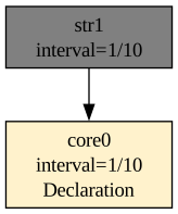
Fig. 33. Ephemeris–artifact dependency
Let’s make this graph a bit more complex by adding two ephemeris declarations and an additional artifact.
DECLARE a UINT STREAM core0, 0.1 TEXTFILE 'datafile1.txt'
DECLARE a UINT STREAM core1, 0.1 TEXTFILE 'datafile2.txt'
SELECT str1[0] STREAM str1 FROM core0
SELECT str2[0] STREAM str2 FROM core0 + core1
The dependency graph for the set of queries above looks as follows (Fig. 34):
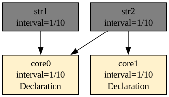
Fig. 34. Ephemerides–artifacts dependency
Let’s build an additional node that depends on artifacts. The simplest way is to add the following query at the end:
SELECT str3[0] STREAM str3 FROM str1#str2
The graph changes shape:
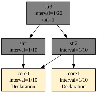
Fig. 35. Ephemerides–artifacts–artifacts dependency
As shown in Fig. 35, the str3 stream is not directly dependent on the data supplied by the core0 and core1 streams. Queries form a dependency graph, and the order in which they are invoked is well-defined. The interval value of streams grows toward the roots. This growth toward the roots follows from the interval-determination equations of the developed algebra.
Note that queries in the rql file are processed sequentially. Attempting to reference, in a query, an object that is not yet defined results in a compilation error.
Attaching the following query to the dependency tree produces an additional substrate.
SELECT str4[0] STREAM str4 FROM (core1+core0)>2
A query attached this way will modify the dependency tree as shown in Fig. 36.
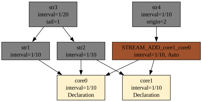
Fig. 36. Dependency with a substrate
The substrate is marked with a different color and an “Auto” label next to the time interval.
The dependency graph must be a directed acyclic graph (DAG). Attempting to define a stream that refers to its own results creates a cycle and results in a compilation error. The detection mechanism is described in the chapter Loop Detection in Compilation.
NOTE: The functionality described here is covered by the test:
subquery, described in the appendix Integration Tests.
Substrates
I mentioned substrates, ephemerides, and artifacts in the chapter on system architecture. Here I’ll present an example.
First I’d like to draw attention to a certain property of the algebraic expressions introduced. In practice we can write any expression, compile it, and produce a formula for operations on individual elements of the time series that yields the desired result.
In practice, the system carries out only one- or two-argument operations. Examples of one-argument operations are the time shift or the Agse operation - there, the argument is a single data stream. The rest of the operations act on two data streams. During compilation, all algebraic expressions are broken down into ones with two arguments.
The parser accepts both the parenthesized form and unparenthesized chains, e.g. s1+s2+s3, s1#s2#s3, and s1+s2+s3+s4. Such notation is then reduced to a sequence of two-argument operations with automatic intermediate substrates.
The example uses the canonical declarations from the whole chapter - three streams with different types and intervals:
DECLARE a BYTE, b INTEGER STREAM core0, 0.1 TEXTFILE 'sensor_a.txt'
DECLARE c INTEGER, d FLOAT STREAM core1, 0.2 TEXTFILE 'sensor_b.txt'
DECLARE e INTEGER STREAM core2, 0.3 TEXTFILE 'sensor_c.txt'

SELECT merged[0] STREAM merged FROM (core0 # core1) + core2
Compilation:
core0(1/10)	sensor_a.txt
	a: BYTE
	b: INTEGER
core1(1/5)	sensor_b.txt
	c: INTEGER
	d: FLOAT
STREAM_HASH_core0_core1(1/15)	tail=2
	:- PUSH_STREAM(core0)
	:- PUSH_STREAM(core1)
	:- STREAM_HASH
	a: INTEGER
		PUSH_ID(STREAM_HASH_core0_core1[0])
	b: FLOAT
		PUSH_ID(STREAM_HASH_core0_core1[1])
core2(3/10)	sensor_c.txt
	e: INTEGER
merged(1/15)	tail=4
	:- PUSH_STREAM(STREAM_HASH_core0_core1)
	:- PUSH_STREAM(core2)
	:- STREAM_ADD
	merged_0: INTEGER
		PUSH_ID(merged[0])
An unannounced stream, STREAM_HASH_core0_core1, appeared - this is exactly a substrate. The compiler broke (core0 # core1) + core2 into two two-argument operations and inserted an intermediate stream. The substrate’s delta: Δ = (1/10 · 1/5) / (1/10 + 1/5) = 1/15.
What happens once we attach the query:
SELECT merged2[0] STREAM merged2 FROM (core0 # core1) > 2
Only one new query gets attached to the plan:
core0(1/10)	sensor_a.txt
	a: BYTE
	b: INTEGER
core1(1/5)	sensor_b.txt
	c: INTEGER
	d: FLOAT
STREAM_HASH_core0_core1(1/15)	tail=2
	:- PUSH_STREAM(core0)
	:- PUSH_STREAM(core1)
	:- STREAM_HASH
	a: INTEGER
		PUSH_ID(STREAM_HASH_core0_core1[0])
	b: FLOAT
		PUSH_ID(STREAM_HASH_core0_core1[1])
core2(3/10)	sensor_c.txt
	e: INTEGER
merged(1/15)	tail=4
	:- PUSH_STREAM(STREAM_HASH_core0_core1)
	:- PUSH_STREAM(core2)
	:- STREAM_ADD
	merged_0: INTEGER
		PUSH_ID(merged[0])
merged2(1/15)	origin=2
	:- PUSH_STREAM(STREAM_HASH_core0_core1)
	:- STREAM_TIMEMOVE(2)
	merged2_0: INTEGER
		PUSH_ID(merged2[0])
You’re probably wondering why only one, and not two again? The answer is optimization. We’re reusing the intermediate results from before. This is one of the unexpected benefits of using RetractorDB.
There’s one more important thing worth mentioning here. There is a SUBSTRAT directive, whose argument is a string in quotes. You can use the following types: ‘memory’, ‘default’, ‘direct’, ‘posix’, ‘posixshd’, ‘generic’, ‘device’, ‘textsource’. A full description of each type can be found in the chapter Storage Types. The default type, ‘default’, causes substrates to materialize entirely on disk. That’s not the desired behavior in a production system, but it is desired during development and debugging. A useful type is ‘memory’. Substrates of this type live only in memory. Their data never lands on disk - everything happens in memory, and there’s only as much data as is needed to execute the queries. The remaining types are currently untested and in development.
Adding a query with the same operations but a different name can trigger substrate deduplication. If the program, delta, and schema are equivalent, the compiler redirects the PUSH_STREAM references to the existing stream and removes the duplicate.
NOTE: The functionality described here is covered by the tests:
issue96_no_substrat_reduction,issue96_substrat_reference, described in the appendix Integration Tests.
Substrate reduction
The compiler carries out an optimization called substrate reduction (the deduplicateSubstrats function). It works as follows: if the user has defined a query structurally identical to a generated substrate, the substrate is removed from the plan and its references are replaced with the user query’s name.
Conditions for reduction
Reduction of a substrate into a user query happens if and only if three conditions are simultaneously satisfied:
- The same schema shape - the field count, types, byte sizes, and cardinalities are identical. Field names are not compared.
- The same delta - the streams’ sampling rate is the same.
- The same processing operations - the sequence of
PUSH_STREAM/STREAM_TIMEMOVE/STREAM_HASH, etc. instructions is identical.
Reduction example
Consider a query with the canonical declarations:
DECLARE a BYTE, b INTEGER   STREAM core0, 0.1 TEXTFILE 'sensor_a.txt'
DECLARE c INTEGER, d FLOAT  STREAM core1, 0.2 TEXTFILE 'sensor_b.txt'

SELECT merged[0]  STREAM merged  FROM (core0 > 2) + core1
SELECT shifted[0] STREAM shifted FROM core0 > 2
Without reduction, the compiler would generate three streams: the substrate STREAM_TIMEMOVE_core0, merged, and shifted. The substrate and shifted have an identical structure - the same source stream core0 and the same >2 operation. After reduction, the substrate is removed, and the reference PUSH_STREAM(STREAM_TIMEMOVE_core0) inside merged is replaced with PUSH_STREAM(shifted):
core0(1/10)	sensor_a.txt
	a: BYTE
	b: INTEGER
STREAM_TIMEMOVE_2_core0(1/10)	origin=2
	:- PUSH_STREAM(core0)
	:- STREAM_TIMEMOVE(2)
	a: BYTE
		PUSH_ID(STREAM_TIMEMOVE_2_core0[0])
	b: INTEGER
		PUSH_ID(STREAM_TIMEMOVE_2_core0[1])
core1(1/5)	sensor_b.txt
	c: INTEGER
	d: FLOAT
merged(1/10)	tail=1	origin=2
	:- PUSH_STREAM(STREAM_TIMEMOVE_2_core0)
	:- PUSH_STREAM(core1)
	:- STREAM_ADD
	merged_0: BYTE
		PUSH_ID(merged[0])
shifted(1/10)	origin=2
	:- PUSH_STREAM(core0)
	:- STREAM_TIMEMOVE(2)
	shifted_0: BYTE
		PUSH_ID(shifted[0])
An important restriction: only substrates are reduced
Reduction applies exclusively to substrates generated by the compiler (isSubstrat = true). Queries explicitly defined by the user are never reduced, even if two of them have an identical structure.
Example - two user queries with the same operation:
DECLARE a BYTE, b INTEGER   STREAM core0, 0.1 TEXTFILE 'sensor_a.txt'

SELECT shifted1[0] STREAM shifted1 FROM core0 > 2
SELECT shifted2[0] STREAM shifted2 FROM core0 > 2
The compilation result keeps both streams, with no reduction at all:
shifted1(1/10)
        :- PUSH_STREAM(core0)
        :- STREAM_TIMEMOVE(2)
        shifted1_0: BYTE
                PUSH_ID(shifted1[0])
shifted2(1/10)
        :- PUSH_STREAM(core0)
        :- STREAM_TIMEMOVE(2)
        shifted2_0: BYTE
                PUSH_ID(shifted2[0])
core0(1/10)     sensor_a.txt
        a: BYTE
        b: INTEGER
This semantic decision is deliberate: the user declared two separate output streams, and both are entitled to exist independently in the execution plan. The deduplicateSubstrats() pass removes neither of them. The compiler may, however, share their internal computation while retaining both public streams, as described in the next section.
Sharing equivalent SELECT computations
The shareEquivalentSelectComputations() pass detects explicit SELECT queries that execute the same field program over equivalent FROM trees containing STREAM_ADD. Instead of executing the expensive program separately for each query, the compiler creates one STREAM_SELECT_* substrate. The public streams remain in the plan as lightweight projections of that substrate.
Example:
SELECT a[_] * b[_] STREAM c1 FROM a+b
SELECT a[_] * b[_] STREAM c2 FROM b+a
After field references are resolved, both field programs read the same values from a and b, even though the stream + operator builds its input in a different order. The plan contains one shared computation, for example STREAM_SELECT_c1, and two public streams, c1 and c2, that read its fields.
Equivalence conditions
Two queries may share a computation only when:
- they have the same result interval;
- they have the same number and order of result fields;
- corresponding fields have the same type, size, and cardinality;
- after field references and
[_]are expanded, the field programs read the same source fields and execute the same operations in the same order; - the
FROMtrees are equivalent while preserving their grouping.
The tree fingerprint canonically orders the two children of each individual STREAM_ADD node, so a+b may be equivalent to b+a. It does not flatten the tree or assume associativity. This matters for three sources with different intervals:
SELECT p[_] * q[_] + r[_] STREAM x1 FROM (p+q)+r
SELECT p[_] * q[_] + r[_] STREAM x2 FROM (q+p)+r
SELECT p[_] * q[_] + r[_] STREAM x3 FROM (r+q)+p
Queries x1 and x2 may share their computation because they swap only the children of the same inner node. Query x3 has different grouping and a different intermediate substrate; its execution cadence may differ, so it remains independent.
Input order is also observable through a full scan and through projection order. The following pairs must not be merged:
SELECT *          STREAM d1 FROM a+b
SELECT *          STREAM d2 FROM b+a
SELECT a[0], b[1] STREAM n1 FROM a+b
SELECT b[1], a[0] STREAM n2 FROM b+a
Preserving the public contract
The optimization shares only the internal computation. Every explicit stream retains its own name, schema and descriptor, rules, retention, storage policy, and artifacts. Automatically generated field names may therefore still differ between c1 and c2, even when their data is identical. This is not a full alias: no public stream disappears from the plan, IPC, or storage.
After creating the common STREAM_SELECT_*, the compiler removes orphaned substrates to a fixed point. During ad hoc import, analysis is restricted to new identifiers so recompilation cannot rewrite streams that have already been instantiated in the live plan.
The pass runs after resolveFieldReferences() and expandIndexWildcards(), but before localizeFieldOffsets(). This lets a field fingerprint compare the source identity and index instead of a local offset that depends on whether the input order is a+b or b+a.
The select_cse_commutative_add test checks both plan shape and execution. It covers equivalent indexed projections and explicit field lists, NULL values and their metadata, separate public descriptors, SELECT *, changed field order, and positive and negative three-source cases. The test compares equivalent pairs byte for byte and confirms that the counterexamples produce different results - see Integration Tests.
Elimination of duplicate substrates
When several queries use the same stream operation - e.g. core0 + core1 - the substrate-extraction phase (extractIntermediateStreams) creates a separate substrate for each of them. Without a subsequent repair phase, the graph would end up with parallel, identical intermediate nodes computing exactly the same value.
When a substrate is created
A substrate is generated for every query whose program contains more than one stream operator. This applies to the operators: STREAM_ADD, STREAM_SUBTRACT, STREAM_HASH, STREAM_DEHASH_DIV, STREAM_DEHASH_MOD, STREAM_TIMEMOVE, STREAM_AGSE. The condition is checked by the query::isReductionRequired() function.
The newly created substrate is given a name built from the operation symbol, its parameter, and the operand names, for example STREAM_ADD_core1_core0, STREAM_TIMEMOVE_2_core0, or STREAM_AGSE_1_10_core0 (the composeStreamName function in compiler.cpp). A parameter is part of node identity: two different windows over one source must not receive the same name. Characters unavailable in identifiers are encoded; a negative number uses N, for example, and a fraction slash becomes _.
A readable name grows with the complexity of the FROM clause and is also the substrate’s file name. Above 200 bytes the compiler keeps the operation name and replaces the remainder with a stable 16-digit FNV-1a digest, for example STREAM_ADD_x92741c15f69ba93f. This lets a wide expression stay below the system NAME_MAX; the same plan structure always receives the same name, while a different operand order receives a different digest. validateSubstratNameUniqueness() stops compilation if one digest were ever to denote two different programs.
In the parent query’s program, the operator token is replaced with a PUSH_STREAM token pointing at this substrate.
Matched interleave-shift factorization
After extracting substrates and resolving their intervals, the compiler applies the algebraic rewrite:
\[ (A > i) \mathbin{\#} (B > k) \longrightarrow (A \mathbin{\#} B) > (i+k), \qquad i\Delta_{a}=k\Delta_{b} \]
The condition \(i\Delta_{a}=k\Delta_{b}\) means that both interleave arguments are shifted by the same physical time. Without this condition the transformation is not equivalent, so the compiler keeps the original plan.
Let the reduced ratio \(\Delta_a/\Delta_b\) be \(p/q\). The interleave tail protects every phase of the period \(p+q\), because the compiler scans that period slot by slot and takes the maximum required latency - formula and justification in Formal Foundations and Proofs.
A shift delays a causal realization: it moves the logical origin O by N and sets its own tail to \(\max(0,W_S-N)\) - it does not change the record sequence or insert a prefix. For \(\Delta_c=\Delta_a\Delta_b/(\Delta_a+\Delta_b)\), the matching condition gives exactly:
\[ \frac{i\Delta_a}{\Delta_c} =\frac{k\Delta_b}{\Delta_c} =i+k \]
Shifting each input therefore corresponds to the same number i+k of output slots, and the logical origin of both sides is identical. The tails are not identical. The factored side reads content directly from the interleave, while the unfactored side reads it only after shifting its components, so it waits longer:
\[ W_{\mathrm{RHS}}=\max\left(0,;W_{\varphi(A,B)}-(i+k)\right)\le W_{\mathrm{LHS}} \]
The rule thus preserves the emitted sequence, the interval and origin=, and may decrease tail=. It is a latency optimization, not a neutral rewrite; for the full proof and a counterexample see Formal foundations and proofs.
Before optimization the plan contains two substrates:
STREAM_TIMEMOVE_i_A = A > i
STREAM_TIMEMOVE_k_B = B > k
result = STREAM_TIMEMOVE_i_A # STREAM_TIMEMOVE_k_B
After optimization only one remains:
STREAM_HASH_A_B = A # B
result = STREAM_HASH_A_B > (i + k)
The factorMatchedHashTimeMoves() pass does not remove explicit user streams or substrates used by other consumers. It runs before deduplication so that the exposed A # B substrate can subsequently be shared with another equivalent plan.
The issue202_hash_shift_e2e test executes both sides of the identity over independent copies of file-backed input streams. It compares the matched and CC artifacts byte for byte, compares their metadata after excluding the reserved header, checks the complete sequence against a reference derived from the B,A,A interleave period, and verifies equal tails (origin=3 with a zero tail - \(\tau_3\) over an interleave of tail 2 absorbs it entirely). Both sides are factored to the same shape here, so the comparison is exhaustive. Neither side emits placeholder records. Separately, computeRequiredCapacities() assigns N+1+2 history records to a declared source: N+1 for the read range itself and two for the declaration’s head lead, which logical-index addressing does not shorten.
The r1_identity_nulls test checks the same identity for \(\Delta_a/\Delta_b=3/2\), which requires the phase maximum \(H_{a,b}=2\) even though the first phase requires only one slot. It compares the rewritten plan, a left-hand side blocked from rewriting, and an explicit right-hand side. The rewritten plan and the explicit right-hand side are equal in full. The blocked left-hand side has the same logical origin and the same content but a strictly larger tail - the comparison therefore covers the common prefix of the payload and of the NULL map, with a separate assertion requiring the factored side to be strictly longer. A nonempty periodic all-NULL record prevents missing data from masking an incorrect tail. Compiler unit tests also cover the \(3/5\), \(7/11\), and \(160/147\) ratios.
The deduplication algorithm
After extracting substrates and determining time intervals, the compiler runs the deduplicateSubstrats() step. The algorithm works iteratively - a while(changed) loop repeats the search until no more duplicate pairs are found.
On every pass, for each pair of substrates (it, it2), five equivalence conditions are checked in turn:
- Time interval –
it->rInterval == it2->rInterval - Program length – the number of tokens in
lProgrammust be identical - Schema length – the number of fields in
lSchemamust be identical - Program content – every token is compared by instruction type (
getCommandID()) and parameter value (getVT()) - Schema content – every field is compared by type (
rtype), size in bytes (rlen), and cardinality (rarray)
If all conditions hold, substrate it is considered a duplicate of substrate it2. The compiler walks through the entire coreInstance and, in every PUSH_STREAM token referring to the old name (it->id), substitutes the new name (it2->id). The duplicate is then removed from the query list (coreInstance.erase(it)), and the loop starts over.
Position in the compilation pipeline
Deduplication is the ninth of the twenty-three pipeline stages (the compiler::compile() function):
checkFunctionCalls- scalar-function names and aritycheckStreamReducerFieldRefs- stream reducer outside theFROMclauseexpandStreamGenerators- stream-family expansionsnapshotNamedSourceRefs- snapshot of user-written referencesextractIntermediateStreams- substrate extractionexpandSchemaWildcards- expansion of*and[_]resolveStreamIntervals- time-interval computationfactorMatchedHashTimeMoves- matched interleave-shift factorizationdeduplicateSubstrats- duplicate elimination ← this stepvalidateSubstratNameUniqueness- substrate-name validationresolveFieldReferences- field-reference resolutionresolveWindowAggregates- record-history aggregate groupsinferFieldShapes- result-field shapescheckRuleConditionShapes- computability of rule conditionssimplifyFieldExpressions- field and rule simplificationshareEquivalentSelectComputations- sharing equivalent SELECT computationslocalizeFieldOffsets- field-offset computationcomputeLogicalOrigin- logical-origin computationcomputeStartupLatency- startup-tail computationcomputeRequiredCapacities- required-history computationvalidateConstraints- operator-constraint validationapplyCapacitiesToStreams- capacity applicationtopologicalSort- final producer–consumer order
Matched interleave-shift factorization and deduplication must happen after interval resolution because both operations compare intervals. Deduplication follows the algebraic rewrite so that it can merge interleave substrates exposed by that rewrite.
SELECT computation sharing runs only after field references and [_] have been expanded because it compares completed field programs. It must still precede field-offset localization so equivalent sources do not look different merely because of their order in the local input buffer.
Every rewriting pass (factorMatchedHashTimeMoves, deduplicateSubstrats, and shareEquivalentSelectComputations) is wrapped in verifyUserFieldNamesPreserved(). Field names of public streams are part of the .desc descriptor and must not change because of optimization. The tail is computed only for the final plan. The final topological sort is unconditional because earlier interval sorting can place a faster # consumer before its producers.
Effect on the dependency graph
Consider the queries:
DECLARE a UINT STREAM core0, 0.1 TEXTFILE 'datafile1.txt'
DECLARE a UINT STREAM core1, 0.1 TEXTFILE 'datafile2.txt'
SELECT str4[0] STREAM str4 FROM (core0+core1)>2
SELECT str5[0] STREAM str5 FROM (core0+core1)>3
Both queries require the sum core0+core1 to be computed first.
The extractIntermediateStreams phase creates a separate substrate for each query, producing two identical intermediate nodes in the graph (Fig. 37):
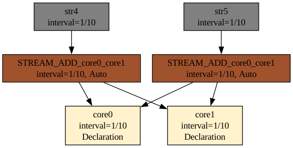
Fig. 37. Graph before deduplication - two identical substrates summing core0+core1
Once deduplicateSubstrats() runs, one of the duplicates is removed and every PUSH_STREAM reference is repointed to the surviving node. A single shared substrate remains in the graph (Fig. 38):
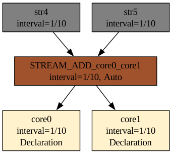
Fig. 38. Graph after deduplication - one shared substrate, generated with: xretractor dedup.rql -c -d
The graph after deduplication is exactly what xretractor -c -d returns - the compiler always presents the result after all optimization phases.
Absorption of a substrate by an explicit stream
The inner loop in deduplicateSubstrats() does not check the isSubstrat flag for candidate it2 - that check exists only in the outer loop. This means an automatic substrate can be absorbed not only by another substrate, but by any stream with an identical program and schema - including a stream explicitly defined by the user.
Consider a query containing only a compound expression:
DECLARE a UINT STREAM core0, 0.1 TEXTFILE 'datafile1.txt'
DECLARE a UINT STREAM core1, 0.1 TEXTFILE 'datafile2.txt'
SELECT str4[0] STREAM str4 FROM (core0+core1)>2
Here, extractIntermediateStreams extracts a substrate STREAM_ADD_core0_core1 for the expression core0+core1. Artifact str4 depends on it (Fig. 39):
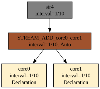
Fig. 39. Graph with the automatic substrate STREAM_ADD_core0_core1
When the user adds an explicit stream declaration that is exactly the same sum:
SELECT * STREAM mysum FROM core0+core1
the substrate STREAM_ADD_core0_core1 satisfies every equivalence condition relative to mysum - identical interval, identical token program, identical field schema. The deduplicateSubstrats() phase removes the substrate and repoints every PUSH_STREAM reference to mysum. The substrate disappears from the graph entirely (Fig. 40):
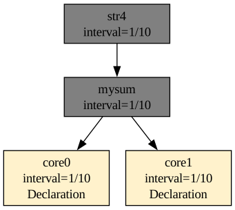
Fig. 40. Graph after adding SELECT * STREAM mysum FROM core0+core1 - the substrate replaced by an explicit stream
A side effect: mysum becomes a shared node - it serves both its own consumers and those that previously used the automatic substrate. In exchange, the user gains an explicit name for the intermediate results and can query them via xqry.
Schema update after absorption
Simply repointing the PUSH_STREAM tokens is not enough. Every stream stores, in lSchema, a sequence of instructions describing how to build the output value of every field - including PUSH_ID(stream_name, N) tokens, which say: “take the N-th field from the input buffer named stream_name.” When a substrate is absorbed, these tokens still refer to the old, removed substrate name. The localizeFieldOffsets() step builds an offset map from the sources of the FROM clause - the PUSH_STREAM tokens in the program and the sources hidden behind compiler substrates - and uses it to turn every PUSH_ID(source, N) into a position in the stream’s own input buffer. A name missing from the map stops compilation with a fatal error, because its position cannot be determined.
Error scenario with a non-zero offset
Consider the query:
DECLARE a INTEGER STREAM s1, 1 BINFILE 'data1.dat'
DECLARE b INTEGER STREAM s2, 1 BINFILE 'data2.dat'
DECLARE c INTEGER STREAM s3, 1 BINFILE 'data3.dat'

SELECT * STREAM mysum  FROM s1+s2
SELECT * STREAM merged FROM s3+(s1+s2)
The compiler creates a substrate STREAM_ADD_s1_s2. Stream merged has two sources: s3 (offset 0) and the substrate STREAM_ADD_s1_s2 (offset 1, because s3 occupies position 0). For the fields that come from the substrate, the buildOutputSchema function writes the following tokens into merged.lSchema:
PUSH_ID(STREAM_ADD_s1_s2, 0)   ← field STREAM_ADD_s1_s2_1 (a from s1)
PUSH_ID(STREAM_ADD_s1_s2, 1)   ← field STREAM_ADD_s1_s2_2 (b from s2)
After absorption, deduplicateSubstrats() repoints PUSH_STREAM from STREAM_ADD_s1_s2 to mysum. Without updating lSchema, however, the PUSH_ID tokens would still carry the old name, which localizeFieldOffsets() cannot find in the offset map. Today this ends compilation with a fatal error. Until 2026-09-14 a missing key silently got offset 0, which is s3’s position - the fields from mysum were then read from offset 0 instead of offset 1, and the compiler gave no warning.
The fix: updating lSchema in deduplicateSubstrats
To avoid this discrepancy, after updating the PUSH_STREAM tokens, deduplicateSubstrats() performs an additional pass over the lSchema of every query and rewrites:
PUSH_ID(old_name, N)tokens intoPUSH_ID(new_name, N)- this covers the fields frombuildOutputSchemaforSTREAM_ADD,PUSH_ID2("old_name[N]")tokens intoPUSH_ID2("new_name[N]")- this covers the symbolic names created bybuildOutputSchemaforSTREAM_TIMEMOVE,STREAM_HASH,STREAM_SUBTRACT.
After the fix, the compiler’s output (xretractor -c) for stream merged from the example above looks correct:
merged(1/1)
        :- PUSH_STREAM(s3)
        :- PUSH_STREAM(mysum)
        :- STREAM_ADD
        s3_0: INTEGER
                PUSH_ID(merged[0])
        STREAM_ADD_s1_s2_1: INTEGER
                PUSH_ID(merged[1])
        STREAM_ADD_s1_s2_2: INTEGER
                PUSH_ID(merged[2])
The fields that come from mysum start at offset 1 (merged[1], merged[2]), which matches mysum’s actual position in merged’s buffer - after field s3_0 from stream s3 at position 0. The fields keep the name of the absorbed substrate: the field names of user streams go into the .desc descriptor, so they are fixed before the optimizations, and the verifyUserFieldNamesPreserved() check makes sure deduplication does not change them.
Cascaded absorption
NOTE: The functionality described here is covered by the tests:
issue167_dedup_cascaded,issue167_dedup_field_names,issue167_dedup_nonzero_offset,issue167_dedup_positive,issue167_triarg, described in the appendix Integration Tests.
deduplicateSubstrats() runs iteratively (while(changed)), which allows for multi-step absorption. In the example:
SELECT * STREAM mysum   FROM s1+s2
SELECT * STREAM shifted FROM (s1+s2)>1
SELECT * STREAM merged  FROM s3+((s1+s2)>1)
in the first round, mysum absorbs STREAM_ADD_s1_s2 and rewrites its names - including in the schema of the intermediate substrate STREAM_TIMEMOVE_1_STREAM_ADD_s1_s2. As a result, in the second round shifted can absorb this substrate (the program condition is now satisfied, because both point to mysum). After two rounds, no automatic substrate remains in the plan, and merged uses s3 and shifted directly.
Asterisk Expansion
Everyone who has written SQL knows the magic * character in that language. Invoking a SELECT command with this argument expands the argument list based on the schemas of the tables produced by relational joins. I wanted to achieve something similar in RQL.
The example uses the canonical declarations used throughout the chapter:
DECLARE a BYTE, b INTEGER STREAM core0, 0.1 TEXTFILE 'sensor_a.txt'
DECLARE c INTEGER, d FLOAT STREAM core1, 0.2 TEXTFILE 'sensor_b.txt'

SELECT *         STREAM merged FROM core0 + core1
SELECT merged[2] STREAM result FROM merged
Let’s compile it and see the effect:
core0(1/10)	sensor_a.txt
	a: BYTE
	b: INTEGER
core1(1/5)	sensor_b.txt
	c: INTEGER
	d: FLOAT
merged(1/10)	tail=1
	:- PUSH_STREAM(core0)
	:- PUSH_STREAM(core1)
	:- STREAM_ADD
	core0_0: BYTE
		PUSH_ID(merged[0])
	core0_1: INTEGER
		PUSH_ID(merged[1])
	core1_2: INTEGER
		PUSH_ID(merged[2])
	core1_3: FLOAT
		PUSH_ID(merged[3])
result(1/10)	tail=1
	:- PUSH_STREAM(merged)
	result_0: INTEGER
		PUSH_ID(result[2])
The * symbol turned into four fields: core0_0, core0_1, core1_2, core1_3. Naming convention: source stream name + absolute position in the output schema. Field types determine the order - core0 contributes BYTE and INTEGER at positions 0 and 1, core1 contributes INTEGER and FLOAT at positions 2 and 3. Referring to merged[2] in the result query gets us a field of type INTEGER - third in order, the first field from core1.
NOTE: The functionality described here is covered by the test:
Pattern3, described in the appendix Integration Tests.
Interval Resolution
Every stream in RetractorDB has an assigned time interval - delta (Δ). The interval determines how often new values are produced. For declared streams (DECLARE), the interval is given by the user. For output streams (SELECT), the interval is determined by the compiler from the stream-algebra equations.
The examples in this chapter use the canonical declarations from the whole chapter: core0 (Δ=1/10), core1 (Δ=1/5), core2 (Δ=3/10).
Algorithm
The resolveStreamIntervals stage works iteratively:
prevUnresolved = ∞
loop:
    unresolvedCount = 0
    sort qTree topologically
    for every query:
        if the source streams' deltas are known:
            determine the output delta from the operator's equation
        otherwise:
            unresolvedCount++
    if unresolvedCount == 0: done (success)
    if unresolvedCount >= prevUnresolved: error (loop in the graph)
    prevUnresolved = unresolvedCount
Every round resolves at least one stream - because the graph is acyclic, and the topological sort guarantees sources are processed before outputs. If the number of unresolved streams stops decreasing, that indicates a cycle - see Loop Detection.
Operator equations
Stream sum (+, STREAM_ADD)
SELECT ... STREAM c FROM a + b
\[\Delta_c = \min(\Delta_a, \Delta_b)\]
The output stream produces values as often as the faster of the input streams.
Example: core0(Δ=1/10) + core1(Δ=1/5) → str1(Δ=1/10)
Stream synchronization (#, STREAM_HASH)
SELECT ... STREAM c FROM a # b
\[\Delta_c = \frac{\Delta_a \cdot \Delta_b}{\Delta_a + \Delta_b}\]
The result corresponds to the harmonic mean of the intervals - the stream only produces a value when both inputs are available at the same time.
Example: core0(Δ=1/10) # core1(Δ=1/5) → str1(Δ=1/15)
Time shift (>n, STREAM_TIMEMOVE)
SELECT ... STREAM c FROM a > n
\[\Delta_c = \Delta_a\]
A shift changes neither the stream’s rate nor its emitted record sequence, but it does change the index at which that sequence appears: record m carries the content of record m-n. It is a causal delay, but its carrier is the logical origin, not the tail - records with an index below n have no definition. The operator’s own tail is non-positive: it equals max(0, W_src − n), because record m-n is older than the current one and therefore all the more available. The plan listing shows both quantities as origin= and tail=; the silent slots are their sum and the runtime emits nothing in them.
Source history requires n+1 records for the read range itself, plus two more for a declared source’s head lead (the record armed when the storage is opened and the zero prefetch), which logical-index addressing does not shorten.
Stream reducers (MAX, MIN, AVG, SUMC)
\[\Delta_c = \Delta_a\]
Reducers operate on a complete stream expression, e.g. AVG(a@(1,10)). They reduce values within a record or a window, but the output stream’s interval stays the same as the source’s. The postfix forms .max, .min, .avg, and .sumc remain backward compatible but are deprecated.
The AGSE algorithm (@(step, window), STREAM_AGSE)
SELECT ... STREAM c FROM a @ (step, window)
\[\Delta_c = \frac{\Delta_a \cdot \text{step}}{\text{windowSize}}\]
AGSE (the Episode Series Generation Algorithm) generates sliding windows. The output interval depends on the step and the window size relative to the source.
De-hash operators (STREAM_DEHASH_DIV, STREAM_DEHASH_MOD)
The inverse operations of # - they determine what interval one of the input streams had, given the result’s interval and the other argument:
\[\Delta_a = \frac{\Delta_c \cdot \Delta_b}{\left|\Delta_c - \Delta_b\right|}\]
Why iteration?
In a query with multiple output streams, one stream may depend on another:
DECLARE a INTEGER STREAM core0, 0.1 BINFILE 'data.dat'
SELECT str1[0] STREAM str1 FROM core0
SELECT str2[0] STREAM str2 FROM str1
In the first iteration round, the compiler determines Δ_str1 = 1/10 (because Δ_core0 is known). In the second round - Δ_str2 = 1/10 (because Δ_str1 is now known). Without iteration, str2 would have to be declared before str1, which would limit the language’s expressiveness.
Loop Detection in Compilation
The query dependency graph must be a directed acyclic graph (DAG). If a query refers - directly or indirectly - to its own results, a cycle is created. The compiler detects this situation and aborts compilation with an error.
NOTE: The functionality described here is covered by the test:
issue95_loopInCompile, described in the appendix Integration Tests.
Example of a loop
DECLARE a BYTE, b INTEGER STREAM core0, 0.1 TEXTFILE 'sensor_a.txt'
DECLARE c INTEGER, d FLOAT STREAM core1, 0.2 TEXTFILE 'sensor_b.txt'

SELECT merged[0]*10, merged[2]+10 STREAM merged FROM core0 + core1
SELECT *                          STREAM agg    FROM MAX(merged)
SELECT *                          STREAM broken FROM merged + broken
The last query defines broken as the result of the operation merged + broken - the stream depends on itself. The dependency graph contains a cycle (Fig. 41):
%% pdf-width: 85%
graph LR
    core0 --> merged
    core1 --> merged
    merged --> agg
    merged --> broken
    broken -->|cycle| broken
    style broken fill:#f66,color:#fff
Fig. 41. A cycle in the query dependency graph
Compilation result
Attempting to compile such a file ends with an error:
$ xretractor brokenQuery.rql -c 2>out.txt
$ echo $?
1
$ cat out.txt
[error] Circular dependency: stream interval resolution stalled with 1
>> unresolved streams
The message "Circular dependency in stream definitions" appears when the resolveStreamIntervals stage detects that the number of unresolved streams has stopped decreasing. For how to run compilation and read error messages, see Compilation Debugging.
Detection mechanism
On every iteration round, the resolveStreamIntervals stage counts the streams for which an interval could not yet be determined (unresolvedCount). In a valid, acyclic graph, this number decreases every round - at least one stream always gets its delta determined. In a graph with a cycle, streams depend on each other mutually and none can obtain a value - unresolvedCount stalls.
if (unresolvedCount >= prevUnresolved) {
    SPDLOG_ERROR("Circular dependency: stream interval resolution stalled with
>> {} unresolved streams",
                 unresolvedCount);
    return std::string("Circular dependency in stream definitions");
}
prevUnresolved = unresolvedCount;
The >= condition (rather than >) guards against false positives: if the count doesn’t decrease by even one, progress is impossible.
How to fix it
Remove the stream’s reference to itself, or to a stream that depends on it. In the example above, the query:
SELECT * STREAM broken FROM merged + broken
should be replaced with a reference to a stream that exists independently of broken:
SELECT * STREAM broken FROM merged + core0
Aliasing
When we join two data streams with the sum operator, a new data schema appears. We can refer to the successive values of this schema through the name of the data stream, indexed sequentially from the start of the schema.
We can, however, also use the names the stream was built from. A value can be pointed to both by the output stream’s name, indexed from the start of the schema, and by the source stream’s name, shifted relative to its join position.
The example uses the canonical declarations used throughout the chapter:
DECLARE a BYTE, b INTEGER STREAM core0, 0.1 TEXTFILE 'sensor_a.txt'
DECLARE c INTEGER, d FLOAT STREAM core1, 0.2 TEXTFILE 'sensor_b.txt'

SELECT merged[0], merged[2], core0[0], core1[0] \
STREAM merged \
FROM core0 + core1
After compilation we get:
core0(1/10)	sensor_a.txt
	a: BYTE
	b: INTEGER
core1(1/5)	sensor_b.txt
	c: INTEGER
	d: FLOAT
merged(1/10)	tail=1
	:- PUSH_STREAM(core0)
	:- PUSH_STREAM(core1)
	:- STREAM_ADD
	merged_0: BYTE
		PUSH_ID(merged[0])
	merged_1: INTEGER
		PUSH_ID(merged[2])
	merged_2: BYTE
		PUSH_ID(merged[0])
	merged_3: INTEGER
		PUSH_ID(merged[2])
merged[0] and core0[0] both end up as PUSH_ID(merged[0]) - they are the same field. But core1[0] - the first field of core1’s schema - ends up as PUSH_ID(merged[2]), not merged[0]. The compiler translated the local index core1[0] into an absolute position in the combined schema: core0 occupies positions 0 and 1, so core1 starts at position 2.
A reference outside the FROM clause
A source alias works only when the sum stands directly in the query’s FROM clause. If the sum has been named by a separate query, the consumer’s field list sees only that named stream:
SELECT *                   STREAM merged FROM core0 + core1
SELECT merged[0], core1[0] STREAM result FROM merged
Compilation ends with the error:
Check result:Stream 'result' refers to 'core1', which is not in its FROM clause. A field list reads only the streams named in FROM: refer to the field by its position in the record of a stream in FROM, or move the reference to a query whose FROM names 'core1'.
merged is a user query with its own interval and buffer, so the compiler does not determine the position of its sources in the result record. The correct form addresses the field by its position in the merged record - core1 starts there at position 2:
SELECT merged[0], merged[2] STREAM result FROM merged
The restriction does not apply to substrates created automatically for a compound FROM clause, e.g. FROM (core0 + core1) > 1: source aliases still work through them.
Index out of range
The index in stream[k] must point to a slot the query actually reads. The compiler rejects an index outside that range instead of producing a plan that reads past the end of the input record. The bound depends on what the name refers to:
| Reference | Bound | Accepted example | Rejected example |
|---|---|---|---|
a stream in the FROM clause | the number of slots that stream contributes to FROM | core1[1] with FROM core0 + core1 | core1[2] |
| a stream behind a window or a reducer | the number of slots after the operator, not the stream width | core0[2] with FROM core0@(1,3) | core0[3]; acc[1] with FROM SUMC(acc) |
the query’s own name in the SELECT list | the width of the FROM input record | merged[3] in STREAM merged FROM core0 + core1 | merged[4] |
the stream’s own name in a RULE condition | the width of the stream’s output record | merged[3] with SELECT * STREAM merged | merged[4] |
Windows and reducers change the slot count: core0@(1,3) contributes three slots although core0 has two fields, and SUMC(acc) contributes one. The same count drives the expansion of core0[_], so a hand-written index and the _ form share one range.
Example messages:
Check result:Stream 'merged': stream 'core1' has 2 element(s)
  in its FROM clause, so 'core1[2]' is out of range
Check result:Stream 'merged': the FROM record of 'merged'
  has 4 element(s), so 'merged[4]' is out of range
Check result:Stream 'merged': rule 'alarm' reads the record of 'merged',
  which has 4 element(s), so 'merged[4]' is out of range
An index folded from $ in a stream generator goes through the same check and produces the same message as a hand-written index.
Aliasing after sum and interleave
The source aliases described above apply to the stream sum operator +. Sum concatenates schemas, so it preserves the position and identity of every component: core0[0] and core1[0] point to different locations in the output record.
The interleave operator # behaves differently. Its two arguments must have schemas of equal cardinality, and the result has one shared schema. In each slot the interleave selects a record from one component, so position k of the left and right arguments becomes the same position k of the result. After A#B, the name A or B can no longer identify the source of the current record.
Comparing compilation for the core0 and core1 declarations above shows the difference without executing the query:
FROM expression | References in the SELECT list | Compilation result |
|---|---|---|
core0 + core1 | core0[0], core1[0] | PUSH_ID(merged[0]), PUSH_ID(merged[2]) - the schemas are concatenated, so the components remain distinguishable |
core0 # core1 | core0[0], core1[0] | compilation error - both arguments share position 0 of the single output schema |
The second row corresponds to this query:
SELECT core0[0], core1[0] STREAM interleaved FROM core0#core1
The compiler stops with a message that core0 is an interleave component and that this reference cannot be distinguished from a reference to the other component. It does not create a plan that silently maps both fields to interleaved[0].
The compiler therefore rejects user-written named references that try to reach an interleave component through #. The restriction covers every form:
- numeric index:
A[0]; - field name:
A.field, and a bare field name resolved toA; - index wildcard:
A[_]; - qualified full scan:
A.*; - the same references in a
RULEcondition and through substrates generated for a compoundFROMclause.
The correct form refers to the only schema that exists after the interleave:
SELECT result[0], result[1] STREAM result  FROM A#B
SELECT result2.*            STREAM result2 FROM A#B
An unqualified * also denotes the complete output schema and remains legal. If a later computation needs [_], name the interleave first and then use its result:
SELECT *                  STREAM interleaved FROM A#B
SELECT interleaved[_] * 2 STREAM scaled      FROM interleaved
When a particular component is needed again, recover it with the de-interleave operator & or % instead of using a source name through a # node.
NOTE: Aliasing after
+is covered by thePattern7integration test, and rejection of a reference outsideFROMby thefield_ref_outside_fromtest. Rejection of named#components and positive controls for the result name are covered byut_compilerunit tests.
Underscore Symbol Processing
The [_] index is syntactic sugar that replicates a field expression. One expression written in SELECT expands during compilation into multiple output fields, one for each compatible slot of the referenced streams.
The number of copies is not determined solely by a stream’s own schema. x[_] denotes all slots that x contributes to the record produced by the query’s complete FROM clause. This distinction matters when a stream operator changes the schema width, for example by creating a window.
The example uses the canonical declarations used throughout the chapter - core0 has two fields (BYTE, INTEGER), core1 has two fields (INTEGER, FLOAT), the schemas have equal cardinality:
DECLARE a BYTE, b INTEGER   STREAM core0, 0.1 TEXTFILE 'sensor_a.txt'
DECLARE c INTEGER, d FLOAT  STREAM core1, 0.2 TEXTFILE 'sensor_b.txt'

SELECT core0[_] * core1[_] STREAM scaled FROM core0 + core1
After compiling:
core0(1/10)	sensor_a.txt
	a: BYTE
	b: INTEGER
core1(1/5)	sensor_b.txt
	c: INTEGER
	d: FLOAT
scaled(1/10)	tail=1
	:- PUSH_STREAM(core0)
	:- PUSH_STREAM(core1)
	:- STREAM_ADD
	scaled_0: INTEGER
		PUSH_ID(scaled[0])
		PUSH_ID(scaled[2])
		MULTIPLY
	scaled_1: FLOAT
		PUSH_ID(scaled[1])
		PUSH_ID(scaled[3])
		MULTIPLY
The _ symbol expanded into two fields: scaled[0] * scaled[2] (i.e. a * c) and scaled[1] * scaled[3] (i.e. b * d). References to core0 and core1 were translated, via aliasing, into absolute positions in the combined schema. The resulting types are INTEGER (BYTE * INTEGER) and FLOAT (INTEGER * FLOAT) - the result of type promotion, described in a separate subchapter.
Width computed from the FROM clause
The one-field stream src contributes five slots when its window src@(1,5) appears in FROM. An FIR convolution can therefore be written without a separate named window stream:
DECLARE value INTEGER STREAM src, 1/500 TEXTFILE 'data.txt'
DECLARE coef INTEGER[5] STREAM filter, 1 TEXTFILE 'coef.txt'

SELECT src[_] * filter[_] STREAM products FROM src@(1,5)+filter
SELECT products[0]        STREAM output   FROM SUMC(products)
The first query expands into five products. It is equivalent to the longer form:
SELECT *                     STREAM window   FROM src@(1,5)
SELECT window[_] * filter[_] STREAM products FROM window+filter
SELECT products[0]           STREAM output   FROM SUMC(products)
In the shorter form, the compiler extracts the window from FROM as a substrate. Such a compiler-generated substrate is transparent when determining the width contributed by src. A user-named stream such as window, however, is a schema boundary, so the longer form refers to window[_], not src[_].
An operator in FROM can also reduce the width. A reducer collapses a window to one slot, so the following src[_] expands only once:
SELECT src[_] STREAM total FROM SUMC(src@(1,5))
If one expression contains several [_] indices, the compiler creates as many copies as the smallest determined width of their contributions. In a typical convolution, the window and the coefficient stream have the same width.
The compiler rejects a reference when the named stream does not occur in FROM, or when its fields do not form a contiguous block there. The latter occurs, for example, for src[_] under a window built over the concatenation (src+other)@(1,5): fields from both sources are repeated together, so no single width can be assigned to src without guessing. Name the subexpression in a separate query and apply [_] to that named result instead.
The _ symbol and interleave
Component aliases such as A[_] are valid for sum +, because sum preserves separate schema segments for both arguments. Do not use this form for a component reached through interleave #:
SELECT A[_] - B[_] STREAM difference FROM A#B
After interleaving, positions A[k] and B[k] are the same position in the shared schema, so this expression does not identify two different values. The compiler rejects the plan instead of silently calculating result[k]-result[k].
To process an interleaved record with _, name the interleave first and then refer to that result:
SELECT *                  STREAM interleaved FROM A#B
SELECT interleaved[_] * 2 STREAM scaled      FROM interleaved
Recovering a particular component requires the de-interleave operator & or %.
This functionality is mainly used in signal-filter algorithms that apply the same operations to corresponding elements of a window and a coefficient vector. It is not required to access RetractorDB’s complete functionality, but it makes such queries significantly shorter. See Signal Filter Implementation for a complete example.
Type Promotion
What happens when we multiply data of type BYTE with data of type INTEGER? RetractorDB follows strict type-promotion rules. Multiplying a BYTE-type field by a value of a field that is of type INTEGER produces a schema field of type INTEGER. This happens at compile time.
At present, RetractorDB supports the following data types:
| Type | Description |
|---|---|
| BYTE | values 0–255 |
| INTEGER | 4-byte values for signed numbers |
| UINT | like INTEGER, for unsigned numbers |
| RATIONAL | rational numbers |
| FLOAT | floating-point numbers |
| DOUBLE | double-precision floating-point numbers |
| STRING | character strings |
STRING and RATIONAL are used in descriptors, conversions, and expressions; their representation and behavior are checked by ut_payload, ut_convertTypes, and integration scenarios. Complex numbers and rational Eisenstein complex numbers remain outside the current set of types.
An example of type promotion in practice - the scaled query from the chapter Underscore Symbol Processing:
SELECT core0[_] * core1[_] STREAM scaled FROM core0 + core1
core0 has fields BYTE and INTEGER, core1 has fields INTEGER and FLOAT. After expanding _, the compiler determines the output fields’ types:
| Expression | Left type | Right type | Result type |
|---|---|---|---|
scaled[0] * scaled[2] | BYTE | INTEGER | INTEGER |
scaled[1] * scaled[3] | INTEGER | FLOAT | FLOAT |
Where the result field type comes from
The type, length, and multiplicity of a field are determined by a single compiler pass - compiler::inferFieldShapes() - which executes the field’s reverse-Polish program on a stack of types, exactly the way expressionEvaluator executes it on a stack of values. The pass runs after field references and window aggregates have been resolved, and before expression simplification, so the descriptor does not depend on any optimizer switch.
Until September 2026 the same question was answered by four local rules, none of which saw the whole expression. The parser started from INTEGER and recognized FLOAT or DOUBLE only when the cast was the last token of the program; a separate pass inferred STRING; the window reduction type was settled somewhere else again. That produced three results inconsistent with the value the engine wrote into the field: SELECT source[0] over a DOUBLE field yielded INTEGER, to_float('2.5') * 2 yielded INTEGER, and to_integer(AVG(x : 10)) + 1 fell back to RATIONAL.
Contract rules
A pure field read preserves the field’s type and length. Reading one element of a numeric array yields a single value, so multiplicity drops to one; STRING[N] is a single slot and keeps its width.
A binary operator (+, -, *, /, ^) yields the type that ranks higher in the order BYTE < INTEGER < UINT < RATIONAL < FLOAT < DOUBLE - with one exception: BYTE with BYTE yields INTEGER. This is not a design decision but a reflection of the language: uint8_t + uint8_t promotes to int in C++, and int is what ends up in the result. The same promotion applies to exact-type exponentiation, because a^k is computed by the same multiplication as the product written out.
A unary operator (-x, NOT x) preserves the argument’s type, except that NOT over a string yields an INTEGER logical result.
Numeric comparisons yield the operand type after normalization, without the BYTE promotion. String comparisons and NOT over a string yield INTEGER 1 or 0. AND and OR take their result type from the left operand, or from the right when the left is NULL; if the selected operand is a string, the result is INTEGER. These operators do not reach the SELECT list: they live in the RULE condition.
Functions share one policy:
| Functions | Result type |
|---|---|
isnull, IsZero, IsNonZero, Length | always INTEGER |
sin, cos, exp | always DOUBLE; rejected over RATIONAL |
Sqrt, tan, log, log2 | argument type; rejected over RATIONAL |
Ceil, Floor, round, trunc | argument type |
Abs, null2zero | argument type |
to_integer, to_float, to_double, to_string | target type |
sin, cos, and exp compute in double and return DOUBLE even for integer arguments. The other mathematical functions compute through double and cast the result back to the argument’s type: Ceil over a DOUBLE field yields DOUBLE, and Sqrt over INTEGER yields INTEGER. Explicit conversions determine the type of their result also when they sit in the middle of an expression: to_float('2.5') * 2 is FLOAT, and to_integer(AVG(x : 10)) + 1 is INTEGER.
Seven functions with an irrational range - Sqrt, sin, cos, exp, tan, log and log2 - do not compile over an argument of type RATIONAL: the compiler rejects the plan and requires an explicit to_double. This matters in practice, because the reducers MIN, MAX, AVG and SUMC yield RATIONAL for integer or rational inputs. The reason, the error message, the reach of the gate (it also covers a RULE ... WHEN condition), and the exception for the rounding functions are described in Field expressions and scalar functions; they are not repeated here, so that the two pages cannot drift apart on the next change.
A record-window aggregate takes its type from the whole program of its argument, passed through the same rule as the stream reducers: an arithmetic source (BYTE, INTEGER, UINT, RATIONAL) reduces to RATIONAL so an average does not lose precision, while FLOAT and DOUBLE stay themselves. Hence MIN(k : 4) over an INTEGER field yields RATIONAL, but MIN(to_double(k) : 4) yields DOUBLE.
NULL is not a type. A field has a type, and a missing value is a marker in the record metadata. An expression that evaluates to NULL on a given record does not thereby change the type of its field. null2zero(x) passes the argument’s type through, and the zero is stored in that very type.
Propagation through the plan
Operators that copy the operand schema - SELECT *, the shift >N, decimation -r, and the de-interleaves & and % - carry the producer’s field shape slot by slot. Stream sum + concatenates both input schemas. The type travels through an arbitrarily long chain of intermediate streams.
Interleave # reconciles both input schemas at each flat position. It selects the higher type, that type’s width for numeric positions, and the greater length for strings. Differing layouts are converted field by field; for example, RATIONAL combined with FLOAT yields FLOAT and can lose precision. Exact index selection by interleave and de-interleave does not reverse type conversion. Byte-for-byte recovery requires a common layout preserving both inputs’ representations.
Operators that synthesize a schema keep their own: the MIN/MAX/AVG/SUMC reducer in the FROM clause yields one field: RATIONAL for an integer or rational source, FLOAT for FLOAT, and DOUBLE for DOUBLE. The @(step, width) window yields fields of the widest type in the source record.
A DECLARE declaration is a contract with the source file and is not subject to inference - no compiler pass modifies it.
Artifact format change
Correct typing changes .desc and the record layout wherever INTEGER used to come out: DOUBLE occupies 8 bytes instead of 4, so it shifts the offsets of the following fields. A stream computed by an older engine version has an artifact with a different layout and will be rejected at startup as an incompatible schema - just as after any other change to the field list. There is no compatibility period: the descriptor now describes what the engine actually writes, whereas before it described something else.
Compilation Debugging
The compiler transforms an .rql file into an execution plan through several stages. The effect of each stage is visible through xretractor’s diagnostic flags. The tools described here let you answer questions like: why does the schema look different from what I wrote? where does this delta come from? why did a substrate appear?
The basic tool: the -c flag
The -c (--onlycompile) flag stops xretractor after compilation and prints the compiled plan to standard output - without starting processing:
xretractor -c query.rql
An exit code of 0 means success. Code 1 means a compilation error. Error messages go to stderr:
xretractor -c query.rql 2>errors.txt
echo $?
Compilation can be invoked even while another xretractor process is already running - the -c flag does not attempt to acquire the execution lock.
How to read the compilation plan
For the canonical query.rql from this chapter, the plan looks as follows:
core0(1/10)	sensor_a.txt
	a: BYTE
	b: INTEGER
core1(1/5)	sensor_b.txt
	c: INTEGER
	d: FLOAT
merged(1/10)	tail=1
	:- PUSH_STREAM(core0)
	:- PUSH_STREAM(core1)
	:- STREAM_ADD
	core0_0: BYTE
		PUSH_ID(merged[0])
	core0_1: INTEGER
		PUSH_ID(merged[1])
	core1_2: INTEGER
		PUSH_ID(merged[2])
	core1_3: FLOAT
		PUSH_ID(merged[3])
result(1/10)	tail=1
	:- PUSH_STREAM(merged)
	result_0: BYTE
		PUSH_ID(result[0])
	result_1: INTEGER
		PUSH_ID(result[2])
	result_2: BYTE
		PUSH_ID(result[0])
	result_3: INTEGER
		PUSH_ID(result[2])
core2(3/10)	sensor_c.txt
	e: INTEGER
Every block has a fixed format:
streamName(delta)
        :- streamOperation(arg)
        outputFieldName: TYPE
                instruction
                ...
| Element | Meaning |
|---|---|
streamName(delta) | The stream’s name and its interval as a fraction: 1/10 = 0.1 s = 10 Hz |
:- PUSH_STREAM(x) | Pushes stream x onto the stream stack; appears once per FROM argument |
:- STREAM_ADD | The stream-sum operator (+ in FROM) |
:- STREAM_HASH | The stream-synchronization operator (# in FROM) |
:- STREAM_TIMEMOVE(n) | Time shift (>n in FROM) |
field: TYPE | An output-schema field, after type promotion |
PUSH_ID(s[n]) | Pushes the value of field n from stream s onto the stack - the effect of aliasing is visible here |
PUSH_VAL(x) | Pushes the constant x onto the stack |
ADD, MULTIPLY, … | An arithmetic operation: pops two arguments off the stack, pushes the result |
Ephemeris blocks (DECLARE) appear at the end of the plan - they contain the field list and the path to the data file.
Aliasing in the plan: if two output fields point to the same PUSH_ID, they are aliases. In the example, result_0 and result_2 are both PUSH_ID(merged[0]) - confirmation that merged[0] and core0[0] are the same position. See Aliasing.
Substrates in the plan: an automatically generated substrate appears as a block with a name like STREAM_HASH_core0_core1 - with no corresponding SELECT in the source file. See Substrates.
Visualizing the dependency graph
Instead of text, you can generate a graph in DOT format and process it with graphviz:
xretractor -c -d -f -t -s query.rql > out.dot && dot -Tsvg out.dot -o out.svg
Available flags that modify the DOT output:
| Flag | Full name | Meaning |
|---|---|---|
-d | --dot | generate DOT output instead of a text plan |
-f | --fields | show stream fields in the graph nodes |
-t | --tags | show individual field programs (requires -f) |
-s | --streamprogs | show stack-instruction sequences in the nodes |
-u | --rules | show RULE rules |
-p | --transparent | transparent background - for embedding in documents |
The graph shows dependencies between streams as edges directed from sources to results. Substrates have a different color than streams explicitly defined by the user. See Dependency Tree Construction.
NOTE: The functionality described here is covered by the test:
issue31_doc, described in the appendix Integration Tests.
Verifying intervals
If an output stream’s delta is unexpected:
- Check the source streams’ deltas - visible in the DECLARE blocks at the end of the plan.
- Check the operator in the FROM clause - every operator has a different delta equation.
Example: core0(1/10) # core1(1/5) gives a delta of 1/15 (the harmonic mean), not 1/10. If you expected 1/10, use + instead of #. Full equations - see Interval Resolution.
Common compilation errors
Invalid literal or interval
A number outside the target type’s range stops parsing with numeric literal ... is out of range in Parse result:. A zero denominator produces fraction ... has a zero denominator, and a zero interval produces interval ... must be greater than zero. This applies to startup files and ad hoc requests; in the latter case the refusal leaves the server running. Correct the number or choose a positive interval. A Circular dependency message indicates a dependency cycle, not a zero interval.
A cycle in the dependency graph
[error] Circular dependency: stream interval resolution stalled with N
>> unresolved streams
A stream refers, directly or indirectly, to itself. Generate the graph via -d - the cycle will be visible as a loop. See Loop Detection.
Unknown stream
A reference to a stream that hasn’t been declared yet. .rql files are processed sequentially - a SELECT cannot refer to a stream defined further down in the file. Move the DECLARE or SELECT earlier.
Schema cardinality mismatch with _
Both streams in the expression core0[_] * core1[_] must have schemas of the same cardinality. Check how many fields each argument has in the plan’s DECLARE blocks. See Underscore Symbol Processing.
Data file unavailable
This error does not appear with -c - the flag verifies the query’s correctness, it does not check whether the data files exist. The file-access error only appears when processing is started without -c.
Query Execution
The execution process is based on a continuous traversal of the query tree, and a sequential, hierarchical invocation of the procedures that build successive stream tuples and successive data schemas.
The description of the algorithm needs to start with the sequencing procedure. In a system executing queries with a variety of values defining the time period between successive created and arriving data, a way to determine successive intervals is needed.
Let’s start by analyzing the following example. Suppose the system has two data streams. One arrives every second, the other every two seconds. The sequencing algorithm should propose a one-second time interval between invocations of the procedure intended for the first stream, and a two-second interval for the second stream. In practice, a one-second time grid will emerge - in which every one-second node is filled with the tuple-building procedure for the first stream, and, on that same time grid, the second stream attaches its procedures every second node.
The time grid determined during compilation is very important - it defines how often, and at what intervals, data streams will be processed, and which nodes will be covered by the generated stream-processing procedures.
Let’s consider a more complex example. Suppose there are three data streams. The first arrives at a rate of ⅓, the second at ½, and the third at ⅔. Determining the grid and placing successive processing procedures requires a more elaborate solution. The value ⅔ can be simplified to ⅓, since there’s a natural divisor between these values. There is, however, no natural divisor between ½ and ⅓. The grid value that gets determined is ⅕. This is the largest possible rational number that, if a grid is built on the rational-number axis, accommodates regular time series with arrival rates of ½ and ⅓.
All streams are overlaid onto the determined grid, and the set of minimal time gaps is determined for the queries with natural multipliers. In our case, the minimal set of time gaps for queries with multipliers (⅓, ½, ⅔) is the set (⅓, ½). The gaps ⅓ and ⅔ will share a time slot on the grid.
Analyzing the discussion below may make clearer the comments, mentioned earlier in the chapter, generated for the swirly program showing the generated marble diagrams.
Query Tree Traversal Algorithm
General overview
The query-tree traversal algorithm is carried out by two cooperating components: dataModel (processing logic) and executorsm (the time loop and IPC). Before entering the main loop, the system performs a zero step, after which it iterates cyclically over the minimal set of time intervals (Fig. 42).
%% pdf-height: 55%
%%{init: {"markdownAutoWrap": false}}%%
flowchart TD
    A([Initialization]) --> B
    B["processZeroStep()<br/>BINFILE and TEXTFILE: bootstrapDeclaration()<br/>Broadcast file declarations"] --> C
    C["TimeLine::getNextTimeSlot()<br/>Determine the next time slot"] --> W
    W["rtAbsoluteSleep()<br/>Wait for the deadline: anchor + slot time"] --> V
    V["DEVICE: snapshot of due sources under the epoch lock<br/>awaitRecords() outside model locks"] --> D
    D["collectAwaitedStreams()<br/>Under epoch and core locks: dueMask_ and dueNames_"] --> E
    E["dataModel::processRows(dueMask_, currentTimeSlot)<br/>Pass 1: declarations - bootstrap and DEVICE publication<br/>Pass 2: non-declarations - computation and write<br/>Pass 3: file declarations - read for the next slot"] --> F
    F["broadcast(dueNames_, formatRow)<br/>Boost IPC queues to xqry clients<br/>Release the epoch lock"] --> C
Fig. 42. The query tree traversal algorithm – general overview
Data structure: qTree
qTree (src/retractor/lib/qTree.cpp) extends std::vector<query> and is a vector of topologically sorted queries. Sorting is done via DFS over the dependency graph built from query.getDepStream() (Fig. 43).
%%{init: {"markdownAutoWrap": false}}%%
graph TD
    A["A (DECLARE)<br/>rInterval=1/3"] --> B["B<br/>SELECT FROM A<br/>rInterval=1/3"]
    A --> D["D<br/>SELECT FROM A,B<br/>rInterval=1"]
    B --> C["C<br/>SELECT FROM B<br/>rInterval=1/2"]
    B --> D
Fig. 43. Example dependency graph for qTree
After the topological sort, the order in the vector is: [A, B, C, D]. Query C, which depends on B, always ends up after B in iteration - this guarantees correctness of the computations.
The getAvailableTimeIntervals() method extracts the unique rInterval values from all queries (excluding compiler directives and zero values) - the result is the input to the TimeLine constructor.
The minimal time grid: TimeLine / CRSMath
TimeLine (src/retractor/lib/CRSMath.cpp) manages rational time intervals. The constructor reduces the set of intervals - removing multiples and keeping only the coprime ones:
Input: {1/2, 1, 4}  →  Output: {1/2}
(1 = 2 × 1/2, so redundant; 4 = 8 × 1/2, so redundant)

Input: {1/2, 1/3}  →  Output: {1/2, 1/3}
(neither is a multiple of the other)
getNextTimeSlot() determines the next slot as min(delta × counter[delta]) over all deltas. The diagram below illustrates the slots for deltas {1/2, 1/3} and the active queries in each of them (Fig. 44):
%% pdf-width: 100%
timeline
    title Time slots for deltas {1/2, 1/3}
    section t = 1/3
        A (rInterval=1/3) : B (rInterval=1/3)
    section t = 1/2
        C (rInterval=1/2)
    section t = 2/3
        A (rInterval=1/3) : B (rInterval=1/3)
    section t = 1
        A (rInterval=1/3) : B (rInterval=1/3) : C (rInterval=1/2) : D (rInterval=1)
    section t = 4/3
        A (rInterval=1/3) : B (rInterval=1/3)
    section t = 3/2
        C (rInterval=1/2)
Fig. 44. The minimal time grid for deltas {1/2, 1/3}
The check isThisDeltaAwaitCurrentTimeSlot(inDelta) returns true when ctSlot_ / inDelta has a denominator equal to 1 (the slot is an integer multiple of the query’s delta).
The zero step: processZeroStep()
Before entering the executorsm::run() loop, dataModel::processZeroStep() is called. It processes file declarations only (BINFILE and TEXTFILE):
for (const auto &q : coreInstance_)
    if (q.isDeclaration() && q.kind != sourceKind::device)
        bootstrapDeclaration(q);
bootstrapDeclaration() switches the buffer from empty to flux, calls revRead(0) and fire(), then checks the armed state. After the zero step, the file declaration’s record is in outputPayload, ready for consumers. File declarations are broadcast under the same epoch lock.
DEVICE has no zero step or broadcast in this phase. Its first record enters the model only at the start of its first due slot, before dependent queries are computed. A file declaration added ad hoc is initialized before consumers in its first due slot, since it did not participate in the zero step.
The main loop: filtering and processing
Slot schedule
Before processing a slot, the loop waits for its deadline \(T_k = T_0 + t_k\). \(T_0\) is the epoch anchor, read from the monotonic clock (CLOCK_MONOTONIC) just before the first slot, and \(t_k\) is the logical time of the slot returned by TimeLine::getNextTimeSlot(). The loop sleeps only for the time remaining until the deadline (rtAbsoluteSleep()), in every clocked mode - with the --realtime option and without it. The deadline is derived anew from the rational axis of the plan with millisecond precision: the fraction of a millisecond is truncated in each deadline separately, so the rounding error does not add up.
- The work time of a slot does not shift the schedule. Computation, rules, and waiting for a
DEVICEsource use part of the period. As long as they fit in the period, the next slot starts at its deadline and the delay does not grow. - A temporary delay is made up. If a slot ends after the deadline of the next one (e.g. a long wait for a
DEVICEor aDO SYSTEMrule), the overdue slots are processed in order and without sleeping until execution catches up with the schedule. The loop then sleeps again until the deadlines of the original grid. No slot or record is skipped, and the processing order does not change. - Sustained overload is not hidden. When the average work time of a slot exceeds its period, the backlog grows without bound: all slots are still computed, in the same order, but later and later relative to their deadlines. The anchor is never moved, so the delay stays visible (e.g. in the
wake_lag_nsprobe). Execution catches up only once the work of the slots again fits in the period with a margin. - Suspending the process leaves a backlog. A process resumed after
SIGSTOPimmediately processes the overdue slots in bursts. On LinuxCLOCK_MONOTONICdoes not advance while the system is suspended; on macOS it does, so there a machine sleep also leaves a backlog to make up.
The anchor belongs to the plan epoch. Accepting a new plan (xqry --reset) builds a new time axis and reads a new anchor, so the new epoch does not inherit the backlog of the previous one. An ad hoc import does not rewind the axis: new intervals join the current axis from their first occurrence after the current slot, and their deadlines count from the same anchor.
The TIMEOUT deadline of a DEVICE source counts from the actual wake-up of the slot, not from its deadline. In --no-clock mode the loop does not sleep at all. The --realtime option does not change the schedule; it only adds SCHED_FIFO scheduling, memory page locking, and CPU affinity (see Command-Line Options - xretractor).
A stop signal (SIGINT, SIGTERM, SIGHUP) that interrupts the loop’s sleep ends the run before the slot whose deadline has not yet come. A sleep interrupted in any other way is resumed until the same deadline, without determining a new period. On Linux a signal sent to the process interrupts the loop’s sleep; on macOS it may reach the communication thread, and then, as with xqry -k, the run ends only after the current period.
NOTE: The slot schedule is covered by the
slot_scheduleintegration test and by theut_executor_rtunit test.
Query filtering: collectAwaitedStreams()
For the current slot, executorsm::collectAwaitedStreams() builds two parallel representations of the due queries:
dueMask_.assign(coreInstancePtr->size(), 0);
dueNames_.clear();
std::size_t position = 0;
for (const auto &q : *coreInstancePtr) {
    if (tl.isThisDeltaAwaitCurrentTimeSlot(q.rInterval)) {
        dueMask_[position] = 1;
        dueNames_.emplace_back(q.id);
    }
    ++position;
}
dueMask_ is a vector of char with the length of the entire plan: an element equal to 1 marks the due query at the same position in qTree. dueNames_ is a vector of std::string_view containing the names of those queries, used for broadcasting. Both vectors retain their capacity between slots.
The mask must describe the same plan layout that processRows() will process. It is therefore built under locks acquired in the order plan_epoch_mutex, then core_mutex; the epoch lock remains held through slot computation and broadcasting. An ad hoc import can change the plan’s topological order, so building the mask before acquiring the epoch lock would violate this invariant. Epoch protection also preserves the lifetime of the name views.
Processing: processRows(dueMask, currentTimeSlot)
dataModel::processRows(std::span<const char> dueMask, currentTimeSlot) acquires core_mutex, checks the mask length, and refreshes the instance-handle table when qTree::planRevision() changes. The handles correspond to positions in the plan, eliminating repeated name lookups during slot computation. Instances are stored in qSet through std::unique_ptr, so changes to the map layout preserve their addresses.
Before calling processRows(), the executor takes a snapshot of due DEVICE sources under a short epoch lock, then calls rdb::awaitRecords() outside model locks. Waiting fills the accessors’ private buffers; data is published to the model only in processRows().
The function performs three passes over the plan, considering only positions marked in the mask (Fig. 45):
%%{init: {"markdownAutoWrap": false}}%%
flowchart TB
    S([processRows - dueMask]) --> P1
    P1["Pass 1 - due declarations<br/>Bootstrap sources in the empty state<br/>DEVICE: publish the current slot's record"] --> P2

    subgraph P2["Pass 2 - due non-declarations in topological order"]
        direction TB
        X0{"Have origin and tail elapsed?<br/>Are inputs available for the first ad hoc record?"} -->|yes| X1
        X0 -->|no| X5([skip query])
        X1["constructInputPayload()<br/>builds input data from FROM"] --> XW
        XW["computeWindowAggregates()<br/>reduces history for SELECT windows"] --> X2
        X2["constructOutputPayload()<br/>evaluates SELECT expressions"] --> X3
        X3["write()<br/>write to disk or memory"] --> X4
        X4["constructRulesAndUpdate()<br/>evaluates RULE clauses"]
    end

    P2 --> P3
    P3["Pass 3 - due file declarations in the armed state<br/>flux, revRead(0), fire()<br/>Read the record for the next due slot<br/>DEVICE is skipped"] --> E([end])
Fig. 45. The processRows algorithm - three processing passes
DEVICE records are published before the current slot’s consumers. File declarations advance to the next record only after consumers, and only in slots due for that source. A query marked in the mask may still emit no result because of its tail or logical origin (origin).
Record-history windows in the SELECT list
If a query contains MIN/MAX/AVG/SUMC(expression : W), computeWindowAggregates() runs after the FROM payload has been built but before output fields are evaluated. For logical index n, it reads records n-(W-1) through n from the named source. A bare field takes the direct flat-slot path; a general expression is evaluated separately against each historical payload.
NULL values are skipped, and a window with no present value stores NULL for all four statistics. Groups with the same source, expression program, and width share one history scan. Their results go to streamInstance::windowValues and become ordinary operands of constructOutputPayload(), so expressions such as 2*MIN(a : 5)+1 and null2zero(AVG(a+b : 5)) are valid.
Broadcasting results: broadcast()
After every processRows(), broadcast(dueNames_, formatRow) is called while the epoch lock is still held - the algorithm is shown in Fig. 46:
%% pdf-width: 85%
%% pdf-height: 60%
%%{init: {"markdownAutoWrap": false, "flowchart": {"nodeSpacing": 25, "rankSpacing": 30, "padding": 6}}}%%
flowchart TB
A([dueNames_]) --> B["printRowValue()<br/>serialize into a<br/>Boost property_tree"]
B --> C{{"clients subscribed<br/>to the stream?"}}
C -->|none| H([skip])
C -->|yes| D["queue brcdbr<id><br/>try_send(data)"]
D --> E{{"queue full?"}}
E -->|no| F([sent])
E -->|"yes - no<br/>receiver"| G["remove the queue<br/>remove id2StreamName_"]
Fig. 46. The broadcast algorithm – distributing results via Boost IPC
printRowValue() builds a structure with the stream name, field count, values, and a null bitmap, serializes it in Boost info format, and sends it via a boost::interprocess::message_queue.
Full example: queries A, B, C, D for deltas
Fig. 47 shows the selection of due queries and the phase order for the plan [A, B, C, D] from the graph in Fig. 43. A is a file source with interval 1/3. The diagram describes the schedule; actual result emission also depends on the query’s tail and logical origin.
%% pdf-width: 85%
%% pdf-height: 65%
%%{init: {"markdownAutoWrap": false, "sequence": {"mirrorActors": false, "messageMargin": 22, "boxMargin": 6}}}%%
sequenceDiagram
    participant TL as TimeLine
    participant ES as executorsm
    participant DM as dataModel
    participant IPC as Boost IPC

    ES->>DM: processZeroStep()
    DM->>DM: A: bootstrapDeclaration() [armed]
    ES->>IPC: broadcast(A)

    TL-->>ES: nextSlot = 1/3
    ES->>DM: processRows([1,1,0,0], 1/3)
    DM->>DM: Pass 2: B, if origin and tail have elapsed
    DM->>DM: Pass 3: A reads the next record
    ES->>IPC: broadcast(A, B)

    TL-->>ES: nextSlot = 1/2
    ES->>DM: processRows([0,0,1,0], 1/2)
    DM->>DM: Pass 2: C, if origin and tail have elapsed
    Note over DM: A is not due - no read
    ES->>IPC: broadcast(C)

    TL-->>ES: nextSlot = 2/3
    ES->>DM: processRows([1,1,0,0], 2/3)
    DM->>DM: Pass 2: B, if origin and tail have elapsed
    DM->>DM: Pass 3: A reads the next record
    ES->>IPC: broadcast(A, B)

    TL-->>ES: nextSlot = 1
    ES->>DM: processRows([1,1,1,1], 1)
    DM->>DM: Pass 2: B, C, D in topological order
    Note over DM: Each query checks origin and tail
    DM->>DM: Pass 3: A reads the next record
    ES->>IPC: broadcast(A, B, C, D)
Fig. 47. Processing schedule for queries A, B, C, D with deltas {1/2, 1/3}
The names next to broadcast denote its dueNames_ argument, rather than a guarantee that each query sends a record. The dependency tree determines computation order in pass 2, and the intervals determine the mask of active nodes. When A is a DEVICE source, it skips the zero step, waits for data before computation of a due slot, and publishes the record in pass 1; pass 3 then skips it.
Algebraic realization - tying the code to the equations
Every key part of the algorithm described on this page is a direct realization of equations from the algebra of regular time series and the formal proofs.
Algebraic operators in SOperations.hpp
The file src/include/SOperations.hpp encodes the algebra operators directly as functions on rational numbers:
| Operator | Symbol | Function in code |
|---|---|---|
| Interleaving | φ | Hash(Δa, Δb, i, retPos) |
| Left-hand de-interleaving | Θ | Div(Δa, Δb, i) |
| Right-hand de-interleaving | ∼Θ | Mod(Δa, Δb, i) |
| Difference | δ | Subtract(Δa, Δb, i) |
| Aggregation and serialization | Ψ | agse(offset, step) |
Each of these functions is a literal translation of the formula from the algebra. Div implements left-hand de-interleaving:
return i + ceilR((i + 1) * deltaA / deltaB);
\[ a_{n} = c_{n+\left\lceil \frac{(n+1)\Delta_{a}}{\Delta_{b}} \right\rceil} \]
Mod implements right-hand de-interleaving:
return i + floorR(i * deltaB / deltaA);
\[ b_{n} = c_{n+\left\lfloor \frac{n\Delta_{b}}{\Delta_{a}} \right\rfloor} \]
Hash implements the test from the definition of interleaving - the condition \(\left\lfloor iz \right\rfloor = \left\lfloor (i+1)z \right\rfloor\) with \(z = \Delta_{b}/(\Delta_{a}+\Delta_{b})\) - and returns the corresponding offset into stream A or B.
The helper functions floorR() and ceilR() operate exclusively on boost::rational<int>, never passing through double. This is a direct realization of the requirement from Theorem 2: an implicit cast to float breaks the assumptions of Fraenkel’s theorem - materialization into floating-point form must be deferred until the floor or ceiling operation is explicitly applied.
TimeLine as the minimal basis of a covering system
The TimeLine constructor determines the primitive set of intervals - removing every delta that is an integer multiple of another delta in the set. An interval is primitive when no smaller interval in the set divides it with a natural quotient. This is the computation of the minimal covering system in the sense of Fraenkel’s theorem: only primitive deltas generate independent Beatty sequences, and only they are needed to determine the complete time grid.
The getNextTimeSlot() method - marked with the comment // MAGIC Warning in the source - generates successive grid points as:
\[ t_{k} = \min_{\delta \in \mathrm{sr}} \left(\delta \cdot \mathrm{counter}[\delta]\right) \]
where sr is the primitive set of intervals, and \(\mathrm{counter}[\delta]\) counts the “hits” recorded so far for each delta. The two-phase loop - first determining the minimum, then incrementing the counters separately - guarantees correct handling of collisions: several deltas can determine the same slot at once.
ℹ️ Info
The
// MAGIC Warningcomment inCRSMath.cpp’s source means the algorithm is correct for a non-obvious reason. Intuition alone is not enough - correctness is guaranteed by Fraenkel’s theorem. Becausesrcontains only primitive intervals (none a multiple of another), the counters for the individual deltas never “get ahead of each other” in a way that would skip or duplicate a slot. A collision - when two deltas point to the same slot - is a legitimate case, handled by the second loop. The “magic” is that the simple formulamin(δ·counter[δ]), with automatic incrementing, is equivalent to a full Beatty-sequence generator for the entire covering system.
isThisDeltaAwaitCurrentTimeSlot() as a Beatty-sequence membership test
boost::rational<int> value = ctSlot_ / inDelta;
return (value.denominator() == 1);
The test checks whether \(t_{\mathrm{slot}} / \Delta \in \mathbb{N}\) - whether the current slot is an integer multiple of the query’s delta. In the language of Beatty-sequence theory: a point \(t\) belongs to the sequence of density \(\Delta\) if and only if \(t/\Delta\) is a natural number. The condition on the denominator equaling 1 follows from boost::rational arithmetic - the fraction is always in reduced form, so a denominator of 1 means exactly an integer, with no rounding involved.
Ad Hoc Queries
By Ad Hoc queries we mean queries directed at a running system. In the typical scenario originally envisioned during system development, the initial working assumption was that a system user would know all the queries and data sources needed to obtain the processed time series.
During development, however, additional scenarios emerged, assuming that the system’s operation should not be interrupted, and that additional queries should be attached to the query execution plan. We call this kind of functionality Ad Hoc queries - attached to the system while it is running, without interrupting its operation.

Fig. 48. Control flow for Ad Hoc queries
Fig. 48 shows the control flow described above. A file with queries and directives is first directed to the xretractor process. Then, through shared memory, the xqry process pulls data from xretractor. Using that same process, we can send a command to the xretractor process. In this command we include the text of the additional query that xretractor should attach to the tree being processed.
What can be attached at run time
The ad hoc channel accepts exactly one SELECT, DECLARE, or RULE statement. Compiler directives and programs containing multiple statements are rejected without changing the active plan.
A syntax error or invalid value is returned to the client with its reason, and the server continues to accept commands. The parser rejects, among other cases, out-of-range numeric literals, a zero denominator, a zero interval (in DECLARE and with &, %, or -), and an empty FILE name. If attachment fails after import, the server restores the previous plan and releases newly claimed stream names and storage files on the bus. The same command can be retried after the cause is fixed.
Before attaching a SELECT whose output is stored on disk, the server checks whether it can open the data file and, for the applicable storage profiles, the .shadow file. This check does not create new files; for a missing file, it checks the parent directory. A refusal returns the reason to the client, such as cannot open output file, without changing the plan. If the directory becomes unavailable after this check, a later failure to open a POSIX or POSIXSHD accessor, or a DEFAULT/DIRECT segment, is also returned as a refusal: the server rolls back the import and new claims on the bus, stays running, and allows the command to be retried. This handling of late open failures does not cover the STORAGE GENERIC profile.
A new source can be declared without stopping a running engine:
$ xqry -a "DECLARE a BYTE STREAM C, 1 TEXTFILE 'data3.txt'"
Exit code 0 with no message means that the declaration was accepted. The declaration receives its logical-index base in its first due slot. If a query attached later needs a window or a time shift, emission waits until the source has accumulated the complete required history. HOLD is not required; it remains an optional directive that delays the physical read. Repeating DECLARE for an existing name is rejected rather than treated as a configuration update.
With multiple live instances, DECLARE alone cannot identify an owner because it has no FROM clause. The target must then be selected explicitly:
$ xqry --server measurements -a "DECLARE a BYTE STREAM C, 1 TEXTFILE 'data3.txt'"
Attaching the first declaration to a server started with an empty plan is not yet supported; the ad hoc channel requires an active data model.
A rule attached at run time may execute only DO DUMP. DO SYSTEM remains available only in the plan file the instance starts from, because exposing it through IPC would let a client run arbitrary shell commands as the server account. The same boundary holds on the xqry --reset channel, which also carries a complete plan but carries no authorship either: a plan with a DO SYSTEM rule is refused there as a whole, unless the operator deliberately sets service.unrestricted = true (→ xqry). The ad-hoc channel refuses unconditionally and does not read that key. The ON target must be an existing stream created by SELECT.
For a historical DUMP -H TO M range, the WHEN condition is first evaluated no earlier than record H+1 after attachment, when the preceding H records were also produced after attachment. For a range without history (H=0), evaluation starts with the first new record. A MEMORY store must have at least H+1 slots; for H > 0 and capacity N <= H, the request is rejected without attaching the rule. Attachment does not enlarge the existing store. See Alerting implementation for details.
xqry --server measurements -a \
  "RULE alarm ON temperature WHEN temperature[0] > 80 DO DUMP -10 TO 5"
On a MEMORY stream, the example above requires at least 11 slots; with capacity 10, the request is rejected.
With multiple instances, the client routes a SELECT according to the owners of streams in FROM, and a RULE according to the stream in ON. A query combining sources from several servers is rejected. New stream names and storage files are claimed on the bus before the active plan is changed, so ad hoc commands cannot overwrite another instance’s resource.
Ad hoc commands extend the current plan. Use xqry --reset file.rql to replace it fully and atomically, including on an idle instance.
Where an ad hoc stream begins
A plan built from the start of system operation numbers records from the logical origin computed by the compiler. A query attached ad hoc has no such history - its first record is the first slot in which the runtime saw it, not slot zero of the plan. The import is atomic: the compiled tree and its stream instances are published under a common lock, and the execution loop rebuilds the timeline without rewinding, even when the new query introduces a new rate to the system. The same lock protects the zero step from collecting declaration names through publishing the first records, so an ad hoc import waits until that step finishes.
NOTE: This behavior is covered by the
issue227_join_alignmenttest (theadhoc-origincase).
Example
We’ll start the example by preparing a simple query:
DECLARE a BYTE STREAM A, 1 TEXTFILE 'data1.txt'
DECLARE a BYTE STREAM B, 2 TEXTFILE 'data2.txt'
SELECT * STREAM str1 FROM A+B
We’ll save the query file under the name qplan1.rql. For the query to run correctly, we also need to prepare the files data1.txt and data2.txt. I suggest filling data1.txt with consecutive numbers from 1 to 6, each on a new line, and filling data2.txt with numbers from 10 to 15. In a directory prepared this way, we run the command:
$ xretractor qplan1.rql
If we previously performed some operations in this directory and created a str1 stream with a different schema, we’ll get an error titled “Error in data descriptor file”. It will also show information about the differences between the two descriptors. In that case, the files str1 and str1.desc should be deleted and the command run again.
The xretractor process will begin processing data. At this point, open another terminal and issue the command:
$ xqry -d
name | duration | size | count | location  | cap
-----+----------+------+-------+-----------+----
str1 | 1        | 48   | 24    |           | 0
A    | 1        | -1   | 3     | data1.txt | 1
B    | 2        | -1   | 2     | data2.txt | 1
This will display, in tabular form, what’s currently being processed in the system - how many bytes have already arrived, which files the data is being read from, and how much data has already been processed. If a more descriptive format is desired, we can issue the following command:
$ xqry -d -y
---
apiVersion: xqry/v1
streams:
  - name: str1
    delta: 1
    size: 214
    count: 107
  - name: A
    delta: 1
    count: 86
    location: data1.txt
  - name: B
    delta: 2
    count: 43
    location: data2.txt
The response is given in YAML form.
To add another query to the system, we need to issue the command:
$ xqry -a "SELECT * STREAM str2 FROM A#B"
A command in this form sends a new query to the xretractor process. No message and exit code 0 mean that it was accepted. The system compiles it and merges it into the query plan tree; on rejection, xqry returns a non-zero code and writes the diagnostic reason.
If we check the system’s state again, we’ll see the following picture:
$ xqry -d
name | duration | size | count | location  | cap
-----+----------+------+-------+-----------+----
str2 | 2/3      | 10   | 10    |           | 0
A    | 1        | -1   | 23    | data1.txt | 1
str1 | 1        | 312  | 156   |           | 0
B    | 2        | -1   | 12    | data2.txt | 1
Or like this:
$ xqry -d -y
---
apiVersion: xqry/v1
streams:
  - name: str2
    delta: 2/3
    size: 7
    count: 7
  - name: A
    delta: 1
    count: 16
    location: data1.txt
  - name: str1
    delta: 1
    size: 298
    count: 149
  - name: B
    delta: 2
    count: 8
    location: data2.txt
Taking a closer look at the queries via the xqry command, we’ll see the following system response for the str1 query:
$ xqry -t str1 -y
---
apiVersion: xqry/v1
stream:
  name: str1
  delta: 1
query: SELECT * STREAM str1 FROM A+B
fields:
  str1.A_0:
    type: BYTE
  str1.B_1:
    type: BYTE
and for the str2 query:
$ xqry -t str2 -y
---
apiVersion: xqry/v1
stream:
  name: str2
  delta: 2/3
query: SELECT * STREAM str2 FROM A#B
fields:
  str2.a:
    type: BYTE
As you can see, the additional query str2 was correctly merged into the existing query execution plan. You can also see that far less data has accumulated compared to str1.
NOTE: The functionality described here is covered by the test:
issue6_adhoc, described in the appendix Integration Tests.
Alerting Implementation
The alerting mechanism (the RULE directive) is an integral part of the main processing loop. It is not a separate background process - rules are evaluated synchronously, in the same time-grid iteration as the SELECT computations. This guarantees that an alert always refers to data that was just computed, not to the previous cycle.
Where RULE sits in the processing cycle
Recall the processRows() function outlined in the chapter Query Tree Traversal Algorithm. For every non-declaration query, four steps are carried out in sequence (Fig. 49):
%%{init: {"markdownAutoWrap": false}}%%
flowchart LR
    A["constructInputPayload()"] --> B["constructOutputPayload()"]
    B --> C["write()"]
    C --> D["constructRulesAndUpdate()"]
Fig. 49. The order of processing steps for a single query
The fourth step - constructRulesAndUpdate() - is exactly where all rules attached to the current query are executed. It is called after the SELECT results have been written to disk, which means a rule always evaluates against a complete, just-computed sample of the stream.
Evaluating the WHEN condition
Every rule contains a list of tokens describing a logical expression (the condition field of the rule struct). At the moment of evaluation, the system:
- Fetches the current query’s
outputPayload- the current sample of the stream. - Passes the condition to the
expressionEvaluator::eval()engine - the same engine that computesSELECTexpressions. - Casts the result to a boolean (
boolCast): any non-zero numeric value istrue, zero isfalse.
If the condition is satisfied, the action associated with the rule is executed (DO SYSTEM or DO DUMP). If not, the rule is skipped with no side effects at all. The full flow is shown in Fig. 50.
%%{init: {"markdownAutoWrap": false}}%%
flowchart TD
    A["New stream sample"] --> B["expressionEvaluator::eval(condition, sample)"]
    B --> C{boolCast}
    C -->|true| D{action type?}
    C -->|false| E([skip])
    D -->|DO SYSTEM| F["system(command)"]
    D -->|DO DUMP| G["dumpManager::registerTask()"]
    F --> H["dumpManager::<br/>processStreamChunk()"]
    G --> H
Fig. 50. Rule evaluation flow
The DO SYSTEM action
The DO SYSTEM invocation is the simplest: the system calls ::system(command) directly on the processing thread. The call is synchronous - xretractor waits for the process to finish before moving on to the next rule.
The command’s exit code is checked:
0- success, no log entry.≠ 0- xretractor logs an error via spdlog with the exit code.- A
system()failure (e.g. no shell available) - logged as a critical error.
⚠️ Warning
The command is executed synchronously. Long-running scripts (e.g. sending large files, network calls with a timeout) will delay the entire processing cycle. In such cases, it is recommended to launch the process in the background:
DO SYSTEM 'my_script &'.
The DO DUMP action - detailed algorithm
DO DUMP is more complex, since it requires gathering data from the past (moments before the event) and from the future (moments after the event). This is handled by the dumpManager class.
- Event -
WHENholds for samplet; the rule callsdumpManager::registerTask() - Phase 1 - writes
|step_back|historical samples from the stream buffer (or sets a delayed start) - Phase 2 - on subsequent iterations
processStreamChunk()appends future samples - End -
dumpedRecordsToGoreaches 0, the file is closed, and the task leaves the queue
Phase 1: historical data (when the task is registered)
At the moment the rule fires - right after the condition is found to be true - dumpManager::registerTask():
- Removes any existing entry at the dump filename (
unlink()) and creates a new file with POSIXopen()using theO_RDWR | O_CREAT | O_EXCL | O_NOFOLLOW | O_CLOEXECflags. It then removes earlier tasks writing under the same filename from the queue and closes their descriptors (see Retention). - If
step_back < 0, reads|step_back|samples from the stream’s historical buffer.
The compiler accounts for the historical DUMP range when calculating the stream’s required capacity. - Writes the historical samples to the file from oldest to newest (i.e. from
step_backto–1). - Computes how many future samples still need to be collected (
dumpedRecordsToGo = |step_forward - step_back| - |step_back|). - If
step_back ≥ 0(a delayed start), it setsdelayDumpRecordsToGo = step_back.
Example: DUMP -3 TO 2
  At registration: write samples t-3, t-2, t-1  (history)
  Still to collect from the future: 2 samples (t, t+1)
  dumpedRecordsToGo = 2
For a rule from the plan file, a DUMP -H TO M range (H > 0) requires at least H+1 records: H historical records plus the current record. The compiler automatically enlarges the STORAGE MEMORY ring to this capacity, including when RETENTION is omitted or specifies a smaller value. A larger explicit RETENTION remains the ring’s minimum capacity. For DEFAULT and DIRECT file stores with bounded retention, the compiler rejects the plan if retention cannot provide H+1 records even immediately after rotation: (segments - 1) * capacity + 1 >= H+1 must hold. This also applies to retention from the [storage] default_retention configuration setting.
For a rule attached ad hoc, the entire history must be produced after attachment. With a DUMP -H TO M range, the rule can first evaluate its WHEN condition on record H+1 after attachment: the preceding H records provide the history, and the new record is the current sample. Without a historical part (H=0), the condition is evaluated on the first new record. A MEMORY stream must retain at least H+1 records; a request reaching further back is rejected without attaching the rule.
Phase 2: future data (subsequent loop iterations)
After registration, the task goes into the bookOfTasks[streamName] queue. On every subsequent iteration of the time grid (when the stream produces a new sample), dumpManager::processStreamChunk() is called:
- For every active task in the queue (
dumpedRecordsToGo > 0):- If
delayDumpRecordsToGo > 0- decrement and skip (start delay). - Otherwise - write the current sample to the file and decrement
dumpedRecordsToGo.
- If
- Once
dumpedRecordsToGoreaches 0 - close the file descriptor and remove the task from the queue.
The full sequence for DUMP -3 TO 2 is shown in Fig. 51.
%% pdf-width: 85%
%% pdf-height: 55%
%%{init: {"markdownAutoWrap": false, "sequence": {"mirrorActors": false, "messageMargin": 22, "boxMargin": 6}}}%%
sequenceDiagram
    participant SI as streamInstance
    participant DM as dumpManager

    note over SI: Sample t - condition TRUE
    SI->>DM: registerTask(stream, {-3, 2, retention=0})
    DM->>DM: Open file dump.tmp
    DM->>DM: Write t-3, t-2, t-1 (history)
    DM->>DM: dumpedRecordsToGo = 2
    SI->>DM: processStreamChunk(stream)
    DM->>DM: Write t → dumpedRecordsToGo = 1

    note over SI: Sample t+1
    SI->>DM: processStreamChunk(stream)
    DM->>DM: Write t+1 → dumpedRecordsToGo = 0
    DM->>DM: Close the file - task complete
Fig. 51. Data-collection sequence for DO DUMP –3 TO 2
The delayed-start case (step_back ≥ 0)
When step_back is non-negative, the dump does not start at the moment of the event, but step_back samples after it:
Example: DUMP 2 TO 5
  At registration: delayDumpRecordsToGo = 2
  Sample t   → skip (delay=2→1)
  Sample t+1 → skip (delay=1→0)
  Sample t+2 → write (dumpedRecordsToGo = 3→2)
  Sample t+3 → write (dumpedRecordsToGo = 2→1)
  Sample t+4 → write (dumpedRecordsToGo = 1→0) - done
Retention (RETENTION N)
Without a RETENTION clause, every trigger of a rule writes its dump under a single name <stream>_<rule>_dump.tmp. With a RETENTION N clause, the first trigger of a rule in an engine run creates _dump_0.tmp, and subsequent file numbers rotate modulo N: _dump_0.tmp, _dump_1.tmp, …, _dump_(N-1).tmp.
A filename must identify a single rule. A plan in which two DO DUMP rules share the stem <stream>_<rule> - e.g. rule b_c on stream a and rule c on stream a_b - is rejected on load, and a rule attached ad hoc with such a stem is refused. The comparison ignores letter case, because on a case-insensitive file system (macOS by default) Ab_r and ab_R are the same file, and plan validity must not depend on the host. The plan author then renames the rule or the stream.
A dump file is always created anew. The engine removes whatever sits under its name - including a symbolic or hard link, which it does not follow - and creates a new file exclusively (O_EXCL | O_NOFOLLOW). A write therefore does not reach the target of a link substituted at the final dump filename. This protection does not cover substitution of parent directories during path resolution; it is not an atomic guarantee of containment within the storage directory. A process that held the previous dump open still sees its old contents. If the file cannot be created, the engine stops with a fatal error naming the file and the cause.
Dump tasks wait in the bookOfTasks queue, one per stream and shared by all of its DO DUMP rules. The queue has no capacity of its own and evicts no tasks: a task ends after collecting its whole range, or when the same rule recreates its file. After creating the new file, registerTask() removes earlier tasks writing under the same name from the queue, and the dumpTask destructor closes their descriptors. A replaced task therefore does not write to a file already detached from the directory, and under each name only the newest trigger collects data.
A rule without RETENTION thus has at most one task in progress, and a new trigger interrupts its previous, unfinished dump. A rule with RETENTION N has at most N tasks: an unfinished dump is interrupted only by the trigger that returns to its file after the numbering wraps, i.e. the N-th next one. Tasks of other rules on the same stream stay untouched - rules do not cut each other’s dumps, including two rules without RETENTION. The number of descriptors open on a stream does not exceed the sum of these limits over its rules.
For every dump to be complete under frequent events, the time to collect a single dump (|step_back| + step_forward cycles) should be shorter than the interval between events multiplied by N (1 for a rule without RETENTION).
Dump file format
The file contains raw binary records with no header at all - every record has the size determined by the descriptor (descriptor.getSizeInBytes()). The format is identical to the format used by stream artifacts, which lets you read it with the xtrdb tool after manually specifying the schema:
$ xtrdb
> storage <path>
> open <stream>_<rule>_dump { <type> <field> }
> list
> quit
The dump contract: values only, no NULL and no gaps
A dump is a headless block of bytes. dumpManager writes payload->span() directly, record after record, and creates no companion file beside it: there is no .desc, so the schema has to be known from outside, and no .meta, so the NULL map and the transmission gaps have nowhere to go. The .tmp extension suggests a working file, but this is the final artifact - no rename follows once the descriptor is closed.
One consequence follows, and it has to be known before a dump is used as input for anything:
| What the engine knows about the record | What the reader of the dump sees |
|---|---|
a field holds NULL - from nullfill, from a transmission gap, from arithmetic overflow, from division by zero | the substitute value of its type: 0 for BYTE, INTEGER, UINT, FLOAT and DOUBLE, 0/1 for RATIONAL, zero bytes for STRING |
a transmission gap preceded the record (a gap entry in the .meta index) | nothing - records lie one after another, with no marker |
| the record does not exist at all, because the requested window reaches deeper than the accumulated history | a zeroed record, indistinguishable from a record whose values are zero |
A zero in a dump file is therefore indistinguishable from a genuine zero, from NULL, and from a record the engine never had. This is not an implementation oversight but the boundary of the format: NULL and the gap are notions of the engine’s interior - they live in the payload’s NULL map and in the .meta index accompanying an artifact, they are stored there and processed there - and the system has, as of today, no uniform way of writing them down on the outside. A dump is a snapshot of values, not a record of what the engine knew.
Where fidelity is required, two other routes do carry the information about absence:
- the stream artifact (
SELECT … STREAM) together with its.metafile -xtrdbprints theNULLmap and the gaps through themetaandmetarawcommands (→ Files); - the client channel
xqry --jsonl, where an absent value is a separate JSONnull, per element of an array field (→ Stream monitoring API).
The null2zero function in a query is not a third route: it turns absence into a zero explicitly and inside the query, which makes it a lossy conversion rather than a way of exporting the information about absence (→ Aggregate operators).
Multiple rules - evaluation order
Multiple rules can be attached to a single stream. All of them are evaluated in a single constructRulesAndUpdate() iteration, in the order they were declared in the .rql file. Every rule is independent - one being satisfied does not affect the evaluation of the others (Fig. 52).
%%{init: {"markdownAutoWrap": false}}%%
%% pdf-width: 100%
flowchart TD
    A["New sample of stream S"] --> R1["Rule 1: WHEN S[0] > 100"]
    A --> R2["Rule 2: WHEN S[0] < 10"]
    A --> R3["Rule 3: WHEN S[0] > 100"]
    R1 -->|true| A1["DO SYSTEM 'notify-send'"]
    R2 -->|true| A2["DO SYSTEM 'echo alarm'"]
    R3 -->|true| A3["DO DUMP -5 TO 5"]
    R1 -->|false| X1([skip])
    R2 -->|false| X2([skip])
    R3 -->|false| X3([skip])
Fig. 52. Independent evaluation of multiple rules on the same stream
Practical limitations and notes
| Situation | Behavior |
|---|---|
| Condition satisfied twice in a row (e.g. a measurement staying above the threshold) | Every sample registers a new DUMP task; without RETENTION, it interrupts the previous unfinished dump of the same rule, with RETENTION N - only the N-th next trigger does |
Two DUMP rules with the same dump filename stem (e.g. b_c on a and c on a_b, including ones differing only in letter case) | The plan is rejected, an ad-hoc rule is refused; rename the rule or the stream |
A DECLARE input stream used as an ON target | Compilation error - rules can only be attached to SELECT streams |
| A rule from the plan file requests records from before the stream began | The historical part of the dump is not shortened; non-existent records are replaced with zeros |
Too few records since attaching an ad-hoc rule (DUMP -H TO M) | The rule waits to evaluate WHEN until record H+1 after attachment; for H=0, it evaluates the first new record |
An ad-hoc rule with history H > 0 on a MEMORY store of capacity N <= H | The request is rejected without attaching the rule; history plus the current record needs H+1 slots |
| Destination file unavailable (missing STORAGE directory) | Critical FatalError - xretractor exits |
| DO SYSTEM returns a non-zero code | Error logged via spdlog; processing continues |
AGSE Sliding Data Window
A sliding data window is a concept widely used in systems that process streams or time series. The idea is to group data into time windows, giving the user the ability to process it in frozen snapshots.
RetractorDB supports this data-processing model through the AgSe operator (Aggregation and Serialization). This operator is two-argument and operates on a stream. Denoted with the @ symbol, it has the form:
stream@(k, w)
where:
- k - the window’s hop (a natural number): by how many source records the window shifts on every step,
- w - the window size (a non-zero integer): how many source fields a single output record contains.
A positive w follows RetractorDB’s historical convention: the newest window field comes first. A negative value means mirrored aggregation - it reverses that order, placing fields in arrival order.
How the output stream’s interval changes
If the source stream has W fields per record and interval Δ, the output stream of the @(k, w) operator has:
|w|fields per output record,- an output interval
Δ_out = (Δ / W) × k.
| Parameters | Effect |
|---|---|
k = |w| | a tumbling window - successive windows do not overlap |
k < |w| | a sliding window - successive windows overlap |
k > |w| | sampling with gaps - some data is skipped |
k = 1, |w| = 1 | serialization - a multi-field record is split into single-element ones |
w < 0 | mirrored aggregation - arrival order, oldest field first |
Typical usage patterns
# serialization: 2 fields → 1 field (interval ÷ 2)
SELECT * STREAM s1 FROM A@(1,1)

# tumbling window: windows of 4 records, no overlap
SELECT * STREAM s2 FROM A@(4,4)

# sliding window: a 5-element window shifted by 1
SELECT * STREAM s3 FROM A@(1,5)

# sampling: every fifth record (skip=5, window=1)
SELECT * STREAM s4 FROM A@(5,1)

# mirrored deserialization: restoring field order
SELECT * STREAM s5 FROM s1@(2,-2)
Visualizing the @ operator
Below is a schematic representation of how source@(k, w) behaves for a single-element stream:
Input data:       0  1  2  3  4  5  6  7  8  9  ...
                  ↓  ↓  ↓  ↓  ↓  ↓  ↓  ↓  ↓  ↓

@(1, 3) - sliding window, hop=1, window=3:
  [2,1,0]  [3,2,1]  [4,3,2]  [5,4,3]  ...

@(3, 3) - tumbling window, hop=3, window=3:
  [2,1,0]           [5,4,3]           ...

@(5, 1) - sampling every 5 elements:
  [0]               [5]               ...

@(2,-2) - mirrored, hop=2, window=2:
  [0,1]    [2,3]    [4,5]    [6,7]    ...
The window is stamped by the interval end: the record with logical index n spans positions n·k−(|w|−1) … n·k, so its newest field lies exactly at position n·k. The window’s logical index therefore denotes the same instant as the source’s logical index, and joining a window with its own source (a FIR pipeline) does not lead the signal. The illustration above shows the sequence of emitted windows; the first of them carries index origin, not zero.
AGSE emits only complete windows. Initial slots in which the window would reach before the start of the source are not records and have no definition - they form the origin= reported in the plan. Slots in which the window is defined but its newest field has not yet been produced form the tail=. A genuine NULL in source data remains an element of the complete window. The formal tail and history capacity bounds are given in Tails, Logical Origins and Operator Observability.
Examples
The subchapters below present concrete uses of the AgSe operator:
- Serialization Example - turning a multi-field record into a sequence of single-element records and back again via mirrored aggregation.
- Moving Average Example - a sliding window as the basis for a signal-averaging filter.
- Window Types - tumbling, sliding, and sampling on the same data stream.
We’ll start by considering the serialization process using the Aggregation and Serialization operator - AgSe.
NOTE: The functionality described here is covered by the tests:
agse1,agse2,agse3,Pattern6, described in the appendix Integration Tests.
Serialization Example
Let’s start by creating a file qplan3.rql with the following content:
DECLARE a BYTE, b BYTE STREAM A, 1 TEXTFILE 'data3.txt'
SELECT * STREAM str3 FROM A@(1,1)
And let’s prepare a file data3.txt with the following content:
$ seq 0 9 | paste - -
0 1
2 3
4 5
6 7
8 9
The last, empty line matters and is significant. After running xretractor qplan3.rql, and in a second window xqry -s str3, we’ll see something like this:
$ xqry -s str3
7
8
9
0
1
2
3
4
5
6
What we’re seeing is an example of serialization. An interesting aspect of the Agse operator, in this case, is also visible in the query execution plan. We can look at it with the command:
$ xretractor -c qplan3.rql -f -p -d > out.dot && dot -Tsvg out.dot -o out.svg
In the out.svg file we’ll see the following query execution plan (Fig. 53):
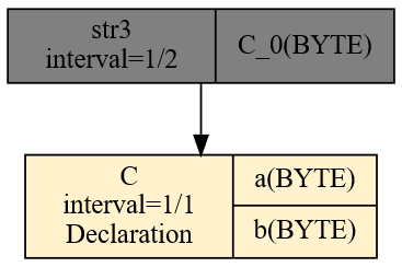
Fig. 53. Query execution plan after AGSE compilation
From a source stream, where data containing two bytes arrives every second, a data stream is created in which one byte appears every half second.
Now that we have a str3 data stream in the system, returning sequential numbers, we can use it for further transformations. Let’s add the following query to the qplan3.rql file:
SELECT * STREAM str4 FROM str3@(2,2)
After running it, though, we won’t see the expected original form of the data3.txt file. Instead, we’ll see something like this:
$ xqry -s str4
2 1
4 3
6 5
8 7
0 9
2 1
4 3
6 5
Along the difficult path of stream processing, there are traps. This is one of them. Only once the reader looks closely will they notice that the data is mirror-flipped. Please change this query to the following form:
SELECT * STREAM str4 FROM str3@(2,-2)
Only a stream built this way will show the original form visible in the data3.txt file:
$ xqry -s str4
3 4
5 6
7 8
9 0
1 2
3 4
That minus sign in the window-width specification is the mirror flip. The window size is two, but the field sequence is built in reverse order.
Generating an image of the query plan that carries out serialization first and then deserialization, we’ll see the following relationship (Fig. 54):
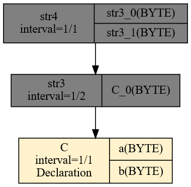
Fig. 54. SErialization and DEserialization
What’s shown here is the most basic example of using the sliding-data-window operator. If we start experimenting with the hop and window size, we’ll notice that we’re able to create an arbitrary sliding window over the data stream, or skip some elements by building a hop larger than the window width.
A recording of the experiment (Animation) looks as follows:
Animation. Session recording of the AGSE serializer experiment
NOTE: The functionality described here is covered by the tests:
agse1,agse2,agse3,Pattern6, described in the appendix Integration Tests.
Moving Average Example
The moving average is one of the simplest and most commonly used signal filters. Every output point is the arithmetic mean of the last N samples. The @(1, N) operator in RetractorDB creates exactly this kind of window: for every new measurement, the last N values are available.
Source data
Let’s assume a temperature stream measured every second. The file temp.txt contains successive readings:
$ seq 10 5 60 > temp.txt
10
15
20
25
30
35
40
45
50
55
60
The RQL query
The file avg.rql:
DECLARE temp INTEGER STREAM sensor, 1 TEXTFILE 'temp.txt'
SELECT * STREAM window5 FROM sensor@(1,5)
SELECT window5[0]+window5[1]+window5[2]+window5[3]+window5[4] \
STREAM sumRow \
FROM window5
SELECT sumRow[0]/5 STREAM avg5 FROM sumRow
What each query does
sensor@(1,5)- creates a sliding 5-element window. Everywindow5record contains the 5 most recent temperature readings. Output interval:1s / 1 × 1 = 1s(hop=1, W=1 field).- Sum of the five fields - a classic
SELECTover the fieldswindow5[0]..window5[4]. - Dividing the sum by 5 - the result is the moving average.
Running it
$ xretractor avg.rql &
$ xqry -s avg5
Example output (the window fills up after the first 5 samples):
30
35
40
45
50
The value 30 corresponds to the average of the first full window: (10+15+20+25+30)/5 = 20… note - RetractorDB does not show partial windows, so the first result to appear corresponds to the moment the window is fully saturated with data.
Verifying the query plan
$ xretractor -c avg.rql -f -p -d > out.dot && dot -Tsvg out.dot -o out.svg
In the generated plan you can see the chain: sensor → window5 → sumRow → avg5. The key node is sensor@(1,5) - from a single-element stream arriving every second, a five-element stream is produced, continuously sliding.
The relationship between window parameters and delay
The moving average introduces a delay of half the window length. For a window of N=5, the delay is 2 samples (2 seconds). Increasing the window:
- reduces noise (more smoothing),
- increases the delay,
- does not change the output interval (with a fixed hop k=1).
Changing the hop with a fixed window:
sensor@(5,5) -- tumbling: a result every 5 seconds, no overlap
sensor@(1,5) -- sliding: a result every second, full overlap
sensor@(3,5) -- partial overlap: a result every 3 seconds
NOTE: The functionality described here is covered by the tests:
agse1,agse2,agse3,Pattern6, described in the appendix Integration Tests.
Window Types
By choosing its two parameters, the @(k, w) operator lets you build every one of the classic window types used in stream processing. Below is a comparison of the patterns on one shared source stream.
Source stream
The file data.txt - 12 consecutive integers:
$ seq 1 12 > data.txt
The source declaration - one record per second, one field:
DECLARE val INTEGER STREAM src, 1 TEXTFILE 'data.txt'
Tumbling window - non-overlapping windows
Hop equal to window size: k = w. Every input element belongs to exactly one output window.
SELECT * STREAM tumbling FROM src@(4,4)
Output interval: 1s × 4 / 1 = 4s. Output records:
$ xqry -s tumbling
1 2 3 4
5 6 7 8
9 10 11 12
Use cases: aggregating samples over fixed time intervals (e.g. per-minute, per-hour).
Sliding window - overlapping windows
Hop smaller than window size: k < w. Every input element appears in several successive windows.
SELECT * STREAM sliding FROM src@(1,4)
Output interval: 1s × 1 / 1 = 1s. Output records:
$ xqry -s sliding
1 2 3 4
2 3 4 5
3 4 5 6
4 5 6 7
...
Use cases: moving averages, trend detection, FIR filters (as in the signal filter implementation).
Sampling - windows with gaps
Hop larger than window size: k > w. Some input elements are skipped.
SELECT * STREAM sampled FROM src@(3,1)
Output interval: 1s × 3 / 1 = 3s. Output records:
$ xqry -s sampled
1
4
7
10
Use cases: signal decimation, sample-rate reduction, diagnostics on every Nth measurement.
Mirrored window - reversed field order
A negative w value reverses the order of fields in the output record, while keeping the same window size.
SELECT * STREAM mirrored FROM src@(2,-2)
Output interval: 1s × 2 / 1 = 2s. Output records (fields in reversed order):
$ xqry -s mirrored
2 1
4 3
6 5
8 7
...
Compare this with src@(2,2), which would give 1 2, 3 4, 5 6… - order matching arrival. Mirrored aggregation is necessary when reversing serialization (deserialization), as described in the serialization example.
Summary of patterns
| Query | Window type | Interval | Record size | Overlap |
|---|---|---|---|---|
src@(4,4) | tumbling | 4 s | 4 fields | none |
src@(1,4) | sliding | 1 s | 4 fields | full |
src@(2,4) | hop window | 2 s | 4 fields | partial |
src@(3,1) | sampling | 3 s | 1 field | none |
src@(2,-2) | mirrored | 2 s | 2 fields | none |
Query execution plan
All four variants can be run at once by placing them in a single .rql file:
DECLARE val INTEGER STREAM src, 1 TEXTFILE 'data.txt'
SELECT * STREAM tumbling FROM src@(4,4)
SELECT * STREAM sliding FROM src@(1,4)
SELECT * STREAM sampled FROM src@(3,1)
SELECT * STREAM mirrored FROM src@(2,-2)
$ xretractor -c windows.rql -f -p -d > out.dot && dot -Tsvg out.dot -o out.svg
The query plan shows four independent branches originating from a shared src node. Each branch implements a different window type with no dependencies between them.
NOTE: The functionality described here is covered by the tests:
agse1,agse2,agse3,Pattern6, described in the appendix Integration Tests.
Stream Playback
We very often think of time series as data marked with timestamps. Data stored, for example, in a file, can be processed however we like - preserving its order based on the recorded time relationships. RetractorDB has been given the ability to re-emit such a stream, preserving the recorded time relationships, as if the data were actually arriving again.
To demonstrate this, let’s prepare a text file filled with data, e.g. from 30 to 45.
$ seq 30 45 > data.txt
We’ll play back a file prepared this way in RetractorDB.
Next, let’s create the following file filled with queries for the system - query.rql, containing only a single declaration ending in HOLD.
DECLARE a INTEGER STREAM core, 1 TEXTFILE 'data.txt' HOLD
In one window, we run the command:
$ xretractor query.rql
In another, we issue the command:
$ xqry -s core
0
0
0
…
We’ll see a sequence of zeros …
In another window we issue the following command:
$ xqry -a "SELECT * STREAM ping FROM core VOLATILE"
Exit code 0 with no message means that the query was accepted. At this point, in the window showing values from the core stream, the core values will appear:
$ xqry -s core
0
0
0
…
0
0
0
30
31
32
33
…
A recorded example below (Fig. 55):
Fig. 55. Recorded example of stream playback
Usage Examples
This chapter presents short examples of using RetractorDB to solve concrete problems encountered when building monitoring systems.
Every example is complete - it includes a problem description, the RQL query design, how to run it, and how to interpret the results. The examples can be run on their own: the required data files and scripts are described step by step.
-
This example demonstrates how to implement a digital FIR filter directly within an RQL query stream, without external DSP libraries. The topic is representative of a broad class of signal-processing problems: noise filtering, frequency-band separation, time-series smoothing.
The example covers:
- designing filter coefficients in GNU Octave (the Remez algorithm, the
remez()method), - transferring the coefficients into a text file and loading them as a
DECLAREstream, - implementing discrete convolution as a set of
SELECTqueries using the sliding-window@operator and expansion of the_symbol, - real-time visualization of the filtering process using
xqryandgnuplot.
The result is a working system that filters a pseudo-random signal (50 Hz) down to the 0–2 Hz band, observed live while xretractor is running.
- designing filter coefficients in GNU Octave (the Remez algorithm, the
-
This example demonstrates using RetractorDB to process clinical ECG signals from the public MIT-BIH Arrhythmia Database (PhysioNet). It’s a complex use case combining several of the system’s mechanisms: multi-channel input streams, a multi-stage FIR filtering pipeline, an adaptive detection threshold, and real-time visualization.
The example covers:
- data preparation: converting MIT-BIH recordings (WFDB format) into text files compatible with RetractorDB,
- implementing the five-stage Pan-Tompkins algorithm in RQL: band-pass filter → differentiation → squaring → moving-window integration → threshold detection,
- visualizing the ECG signal and the QRS-detection result in a gnuplot window (RTL mode - newest samples on the right),
- interpreting the results: RR-interval readings, identifying arrhythmia episodes in MIT-BIH record 205.
The result is a working QRS detector processing a two-channel ECG signal (MLII + V1) at 360 Hz, implemented entirely with RQL queries, with no specialized libraries.
-
This example demonstrates how to build OHLC candles (open, high, low, close) from a regular stream of samples and draw them live together with the samples they were built from. The same construction fits any signal viewed in intervals: quotes, sensor readings, load.
The example covers:
- smoothing noise with the record-window aggregate
AVG(... : 25), - a tumbling window with mirrored aggregation,
@(10,-10), which sets the candle boundaries and the order of its samples, - the
MAXandMINreducers in theFROMclause, and joining a candle with its samples into one record with the+operator, - visualization in the
xqry --gnuplot-ohlcmode, started with theninja candlesticktarget.
The result is a chart of 25 candles of 10 samples, refreshed every 0.2 s, in which every candle stands exactly over the samples it was built from.
- smoothing noise with the record-window aggregate
Signal Filter Implementation
Problems related to digital signal processing include problems related to filtering. The goal of filtering is to separate the information contained within a signal. Usually the goal is to separate the signal from its noise.
Filters can be analog or digital. In this solution, we’ll focus on digital filters. A digital filter is implemented as a sequence of operations on successive data points of the processed signal within a given time window. As a rule, when choosing a digital filter we must decide what compromises we’re willing to accept. In addition, we may run into legal restrictions related to certain algorithms or methods [9].
Designing a filter in Octave
When designing a digital filter, we need to determine what range of frequencies we want to attenuate, and what we want to amplify or leave unaffected. We define these parameters as the stopband and the passband. One tool I know of, used for constructing digital filters, is the GNU Octave program (https://octave.org). With this tool we can generate the coefficients needed to compute a simple digital signal filter.
As an example, let’s take the following values needed to construct a signal filter:
- Input signal sampling rate: 50 Hz
- Passband: 0–2 Hz
- Stopband: 5–25 Hz
An input-signal sampling rate of 50 Hz means 50 samples will appear within a second. In RetractorDB, this means the source signal should arrive at a rate of Delta = 0.02. And the defined data source should support that rate.
For these filter assumptions, the Octave program that builds the signal filter looks as follows:
pkg signal load
filtord = 25 % Filter length
Fs = 50; % Sampling rate 50Hz
FNq = Fs/2; % Nyquist frequency
F1c = 2; % Passband 0 - 2Hz
F2c = 5; % Stopband 5 Hz ->
F3c = 25; % Stopband <- 25 Hz
f=[0,F1c/FNq,F2c/FNq,F3c/FNq]
m = [ 1 , 1 , 0, 0 ]
freqz ( remez(filtord,f,m) );
A file prepared this way should be saved to disk, or pasted directly into the Octave terminal window.
We can display the filter’s floating-point parameters by issuing the command remez(filtord,f,m). We get a graphical representation of the filter by issuing the following command:
octave:1> [h, w] = freqz ( remez(filtord,f,m) );
subplot(2,1,1);
plot (f, m, '', w/pi, abs (h), '');
xlabel('Normalized frequency')
ylabel('gain')
grid on
subplot(2,1,2);
plot(f,20*log10(m+1e-5),'', w/pi,20*log10(abs(h)),'');
xlabel('Normalized frequency')
ylabel('gain (dB)')
grid on
Running the code above in Octave produces the following graphical response (Fig. 56):
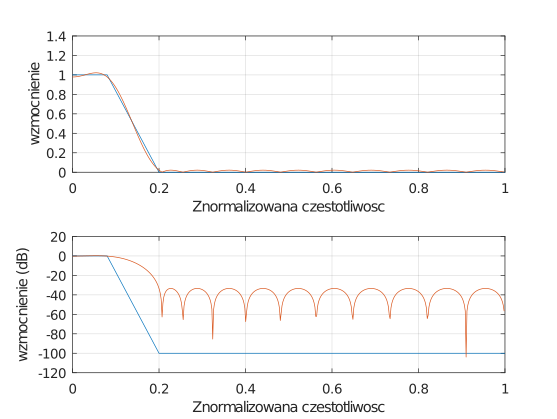
Fig. 56. Graphical representation, in the frequency domain, of the computed digital filter
On the y-axis, Octave shows the normalized frequency. The frequency range shown on the y-axis, from 0 to 1, corresponds to a frequency range of 0Hz to 25Hz. On the x-axis, the first plot shows the linear gain, the second the same quantity but on a logarithmic scale.
The filter’s parameters can be displayed with the command:
octave:11> remez(filtord,f,m)
ans =
-4.2689e-03
-2.0148e-02
-1.4865e-02
-1.8188e-02
-1.4031e-02
-4.5861e-03
…
To get fixed-point parameters for a 16-bit filter, run the command:
octave:12> floor(remez(filtord,f,m) * 32767)
ans =
-140
-661
-488
-596
-460
Implementation in RetractorDB
We should transfer the values obtained into a text file named filterremez.txt.
For testing purposes, we’ll take the source signal from a pseudo-random number generator. We’ll pull the ephemeral data directly from the source at a rate of 50Hz.
The initial part of the query.rql file, containing the source declarations for RetractorDB, looks as follows:
DECLARE coef INTEGER[25] STREAM filter, 1 TEXTFILE 'filterremez.txt'
DECLARE data BYTE STREAM source, 0.02 DEVICE '/dev/urandom'
The next part contains the commands that build the signal-processing pipeline.
SELECT source[_] * filter[_] STREAM accRow FROM source@(1,25)+filter
SELECT accRow[0] STREAM output FROM SUMC(accRow)
SELECT int(output[0]/25/1000),source[0] \
STREAM outputAll \
FROM output+source
The first of these three queries places the window directly in the FROM clause. The source[_] index takes the width of the 25 slots contributed by source@(1,25), so the compiler creates 25 products with the corresponding filter[_] coefficients. A separate named window stream is unnecessary; the compiler extracts it as a plan substrate. SUMC(accRow) then sums the products, and the final query joins the filtered result with the current source sample. The SUMC sum has type RATIONAL, so the final query scales it and casts it to an integer with int(...); without the cast xqry would print fractions such as 2225159/12500, of which gnuplot reads only the numerator, and the filtered trace would fall outside the axis range.
After [_] is expanded, the plan contains many fields, so the full compilation result spans several screens. A compact view of the process can be generated with:
$ xretractor -c query.rql -p -d > out.dot && dot -Tsvg out.dot -o out.svg
We’ll see the following picture (Fig. 57):
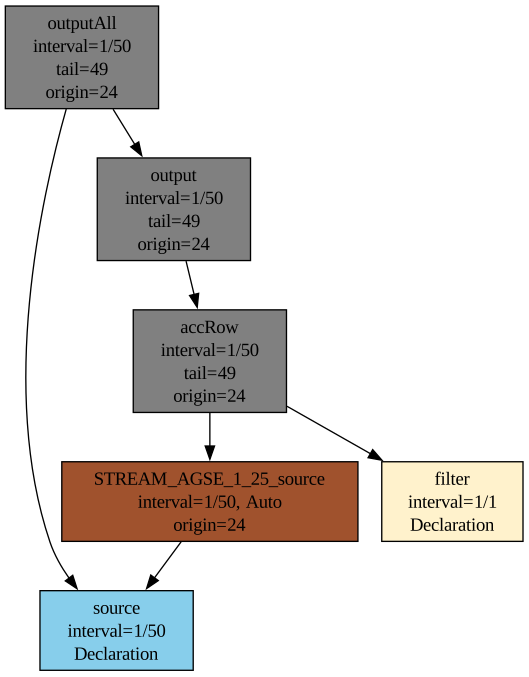
Fig. 57. Dependency between the processed data streams while carrying out the signal filter
Running it
Trying to inspect the contained fields and data types would expand the generated figure so much that it’s impossible to include the generated result here without losing readability.
To watch the signal-processing pipeline in real time, we should issue the following sequence of commands:
- in the first window, start the server process that processes the collected data. The files query.rql and filterremez.txt should be present in this directory, with the command:
$ xretractor query.rql
- in the second window, issue the following command:
$ xqry -s outputAll -p 50:256 | gnuplot
On screen we should see the following chart, running from left to right, continuously filled with data (Fig. 58):
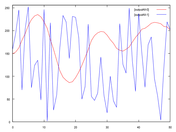
Fig. 58. Signal filtering carried out inside RetractorDB
In Fig. 58 we see two charts overlaid on each other. The more erratic one - shown on screen as a blue line with a lot of variability - is the visualization of the input signal. Data taken from the pseudo-random number generator at a rate of 50 samples per second. And the second chart, wrapping around the input data - shown on screen in red, smoother, flowing around it - is exactly the data filtered by the signal filter we built. A signal whose passband has been restricted to 0–2Hz (low frequencies) and stopped in the region of 5–25Hz (high frequencies). Figuratively speaking, we’ve isolated the bass line.
Keep in mind that, on screen, this chart scrolls to the right very quickly, showcasing the current data-processing capabilities carried out in RetractorDB.
A screen recording during the processing run is shown in Fig. 59:
.gif)
Fig. 59. Animation of the real-time signal-filtering process
NOTE: The functionality described here is covered by the test:
dsp, described in the appendix Integration Tests.
ECG Visualization and Arrhythmia Detection - the MIT-BIH Database
Data source - the PhysioNet MIT-BIH Arrhythmia Database
The MIT-BIH Arrhythmia Database is a publicly available collection of electrocardiogram recordings published by PhysioNet at:
https://physionet.org/content/mitdb/1.0.0/
It contains 48 half-hour, two-channel recordings collected from 47 patients at Beth Israel Hospital in Boston between 1975 and 1979. The recordings were manually annotated by at least two independent cardiologists and are widely used in research on automatic arrhythmia detection.
Record 205
The example uses record 205 - a recording from a 59-year-old man treated with Digoxin and Quinaglute. The record contains episodes of ventricular tachycardia (VT) and is often cited in the literature as diagnostically challenging, due to two morphologically distinct forms of premature ventricular contractions (PVC).
Recording parameters:
| Parameter | Value |
|---|---|
| Duration | ≈ 30 min |
| Sampling rate | 360 Hz |
| Number of samples | 650,000 |
| Channel 1 (MLII) | Modified limb lead II |
| Channel 2 (V1) | Precordial lead V1 |
| Resolution | 12 bits, gain 200 LSB/mV, zero point 1024 |
Raw values are stored as unitless integers (so-called ADC values). Conversion to millivolts:
\[\text{mV} = \frac{\text{ADC} - 1024}{200}\]
The range of actual values in the rec205 file falls between 589–1315 (MLII) and 718–1106 (V1), corresponding to a signal amplitude of roughly ±1.5 mV.
Data preparation
The original recording files (205.hea, 205.dat, 205.atr) are provided in the MIT-BIH format and need to be converted into a binary format recognized by RetractorDB.
The MIT-BIH format 212
The signal in the 205.dat file is packed 12-bit in format 212: every three bytes store two consecutive samples of both channels according to the scheme:
[B0][B1][B2] → MLII = B0 | ((B1 & 0x0F) << 8)
V1 = B2 | ((B1 >> 4) << 8)
The values are 12-bit signed (range –2048..2047).
Converting to the RetractorDB format
The script examples/ecg/mitbih2rdb.py reads the 205.hea header, decodes the sample pairs, and writes them as little-endian int32 records into the rec205 file:
650,000 records × 2 fields × 4 bytes = 5,200,000 bytes
At the same time, the script generates an RQL script that plays back the signal (rec205-replay.rql). The descriptor file rec205.desc is created by build.sh.
The whole preparation process is run with a single command from the project’s root directory:
bash examples/ecg/build.sh
The result is three files in the examples/ecg/rec205/ directory:
| File | Generated by | Description |
|---|---|---|
rec205 | mitbih2rdb.py | Binary data (int32 LE) |
rec205.desc | build.sh | Stream descriptor |
rec205-replay.rql | mitbih2rdb.py | RQL playback script |
The RQL query
The file rec205-replay.rql defines two streams:
DECLARE MLII INTEGER, V1 INTEGER STREAM ecg, 1/360 BINFILE 'rec205'
SELECT ecg.MLII, ecg.V1 STREAM s205out FROM ecg VOLATILE
The STREAM ecg, 1/360 clause sets the time interval of a single sample to 1/360 s, matching the actual sampling rate of 360 Hz. The BINFILE keyword (TYPE BINFILE in the descriptor) causes the rec205 file to be read as raw binary records, sequentially in a loop (after the last sample, reading returns to the beginning), enabling continuous playback of the recording.
The output stream s205out is declared VOLATILE, so it is not written to disk - the data only reaches the consumer process (xqry).
On-screen visualization
The ecg target in the build system is used to display the chart in real time. It runs the script scripts/xplot.sh, which starts xretractor in the background, and then pipes the data stream through xqry into gnuplot.
# from build/Debug
ninja ecg
The invocation CMake expands this into:
scripts/xplot.sh s205out rec205-replay.rql 720,560,1360 --gnuplot-rtl
Meaning of the parameters:
| Parameter | Meaning |
|---|---|
s205out | The name of the output stream |
rec205-replay.rql | The query file |
720 | The data window width (samples visible at once) |
560,1360 | The Y-axis range (ADC values matching the actual signal) |
--gnuplot-rtl | Newest samples on the right, chart scrolls right to left |
The --gnuplot-rtl option is an xqry parameter that reverses gnuplot’s X axis (set xrange [720:0]). The effect is that the freshest samples appear on the right side of the window, and older ones scroll to the left - similar to the classic ECG printout on paper tape.
The script gives the server a name derived from the working directory and passes it to every xqry --server invocation. Several plotting targets can therefore run concurrently without taking over another instance. An optional fifth argument supplies a different name; if that name is already in use, the script exits before removing the output directory.
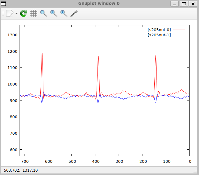
Fig. 60. View of the gnuplot window with the ECG signal being played back (record 205)
The window shown in Fig. 60 displays 720 samples, i.e. exactly 2 seconds of signal at 360 Hz, matching the typical width of a single ECG strip used in diagnostics.
QRS Detection and Arrhythmia Identification
Context - the Pan-Tompkins algorithm
QRS-complex detection is the foundation of automatic ECG analysis. The QRS complex represents ventricular depolarization and corresponds to every heartbeat, visible as a sharp spike in the signal. Knowing the positions of the QRS complexes in time, RR intervals can be computed, and from them, basic rhythm disturbances can be identified:
| Measure derived from QRS | Use |
|---|---|
| RR intervals | Heart rate (HR), VT, bradycardia |
| RR variability (HRV) | Autonomic nervous system, event prediction |
| QRS morphology | Distinguishing PVC from a normal rhythm, APC |
| QRS duration | Bundle branch block (BBB) |
The Pan-Tompkins algorithm (1985) is a classic, five-stage, pipelined digital-signal-processing algorithm implemented with FIR filters. RetractorDB implements it directly as an RQL query stream, without specialized DSP libraries.
Generating the signal filters (coef)
The algorithm requires two sets of FIR coefficients, stored as text files (bp_coef.txt, d_coef.txt). They are generated once, with Python scripts, before running detection.
The band-pass filter - gen_bp_coef.py
Step 1 of the algorithm requires a filter that cuts out noise and artifacts outside the QRS band. A passband of 5–15 Hz at fs = 360 Hz produces a response containing the QRS morphology, while attenuating baseline wander (< 5 Hz) and muscle noise (> 15 Hz).
The design method is a windowed sinc:
h_bp[n] = (h_lp2[n] − h_lp1[n]) · w[n]
where:
h_lp[n] = 2·fc·sinc(2·fc·(n−M))- the ideal low-pass filterw[n] = 0.54 − 0.46·cos(2πn/(N−1))- the Hamming window, damping Gibbs effectsM = (N−1)/2 = 12- the filter’s center point (group delay = 12 samples)
Parameters:
| Parameter | Value |
|---|---|
| Filter length N | 25 coefficients |
| Lower cutoff fc₁ | 5 Hz (normalized 5/360) |
| Upper cutoff fc₂ | 15 Hz (normalized 15/360) |
| Integer scale | ×1000 (divided /1000 in RQL) |
Running the script:
cd examples/ecg/rec205
python3 gen_bp_coef.py
# Saved 25 coefficients to bp_coef.txt
# Coefficients: [-2, -2, -1, 0, 3, 8, 14, 23, 32, 41, 49, 54, 56, ...]
# Sum (DC gain): 5 / 1000 = 0.0050
The coefficients are symmetric about the center (n=12), confirming the filter’s linear phase - an essential property when analyzing ECG, since it guarantees no phase distortion of the QRS morphology.
The differentiating filter - gen_d_coef.py
Step 2 of the algorithm applies a filter that emphasizes the steep edges of the QRS. Pan and Tompkins proposed a 5-point derivative estimator:
y[n] = (1/8T) · (−x[n−4] − 2·x[n−3] + 2·x[n−1] + x[n])
Coefficients (from oldest to newest sample):
h = [−1, −2, 0, 2, 1]
Filter properties:
| Property | Value |
|---|---|
| Sum of coefficients | 0 (zero DC gain - eliminates offsets) |
| Maximum response | f ≈ 10–25 Hz (the QRS-edge range) |
| Scale factor (1/8T) | 360/8 = 45 Hz (ignored - does not affect detection) |
cd examples/ecg/rec205
python3 gen_d_coef.py
# Saved 5 coefficients to d_coef.txt
# Coefficients: [-1, -2, 0, 2, 1]
# Sum (DC gain): 0 (should be 0)
Implementing the pipeline in RQL - rec205-detect.rql
The file rec205-detect.rql implements the complete five-stage pipeline for both ECG channels (MLII and V1):
# Keep windows extracted automatically from FROM in memory
SUBSTRAT 'memory'
DECLARE MLII INTEGER, V1 INTEGER STREAM ecg, 1/360 BINFILE 'rec205'
DECLARE bp_coef INTEGER[25] STREAM bpf, 1 TEXTFILE 'bp_coef.txt'
DECLARE d_coef INTEGER[5] STREAM df, 1 TEXTFILE 'd_coef.txt'
# Extracting the channels
SELECT ecg.MLII STREAM mlii FROM ecg VOLATILE
SELECT ecg.V1 STREAM v1 FROM ecg VOLATILE
# 1. Band-pass filter (5-15 Hz) - 25-tap FIR convolution
SELECT mlii[_]*bpf[_] STREAM bp_acc FROM mlii@(1,25)+bpf VOLATILE
SELECT int(bp_acc[0]/1000) STREAM bp_out FROM SUMC(bp_acc) VOLATILE
# 2. Differentiation - 5-tap FIR convolution
SELECT bp_out[_]*df[_] STREAM d_acc FROM bp_out@(1,5)+df VOLATILE
SELECT int(d_acc[0]) STREAM d_out FROM SUMC(d_acc) VOLATILE
# 3. Squaring (/1000 prevents int32 overflow)
SELECT d_out[0]^2/1000 STREAM sq_out FROM d_out VOLATILE
# 4. Moving-window integration over 30 samples (~83 ms)
SELECT int(sq_out[0]) STREAM mwi FROM AVG(sq_out@(1,30)) VOLATILE
# 5. Adaptive threshold - 2x moving average over 180 samples (0.5 s)
SELECT int(mwi[0]) STREAM mwi_thr FROM AVG(mwi@(1,180)) VOLATILE
# Output: MLII centered, V1 centered, detection signal ×5
SELECT mlii[0]-900, v1[0]-900, (mwi[0]-mwi_thr[0]*2)*5 \
STREAM detect_out FROM mlii+v1+mwi+mwi_thr VOLATILE
Rationale for the parameters
The @(1,25) operator creates a 25-sample sliding window directly in FROM. The mlii[_] index expands according to the 25 slots contributed by this window to the input record, and SUMC adds the products with bpf[_]. The discrete convolution therefore does not require a separate mlii_win query. The same notation creates the five-element differentiating convolution - see Underscore Symbol Processing.
The compiler extracts windows and reducers from a compound FROM clause into compiler-generated substrates. VOLATILE applies to the stream named by a given SELECT, not to these automatic nodes. The SUBSTRAT 'memory' directive keeps the complete intermediate pipeline in memory; without it, the generated windows would use the default on-disk storage.
The bp_acc[0]/1000 division in step 1 compensates for the integer scale of the band-pass filter coefficients. The second /1000, after exponentiation in step 3, limits value growth; without it, d_out[0]^2 could exceed the int32 range (2,147,483,647) for typical ECG amplitudes.
The pipeline computes in integer arithmetic, so every reducer result returns to INTEGER through an explicit int(...) (short for to_integer). SUMC and AVG over an INTEGER field yield RATIONAL; without the cast the denominators grow from stage to stage (/1000, squaring, the 30-sample average) until boost::rational<int> overflows without warning.
The output expression (mwi[0]-mwi_thr[0]*2)*5 implements the adaptive threshold: the value is positive only when the MWI envelope exceeds twice the current moving average - indicating a detected QRS. The ×5 multiplier scales the detection signal to a range visually comparable to the raw ECG on the chart.
Running it - ninja ecg-detect-qrs
The process is started with a single command from the build/Debug directory:
cd build/Debug
ninja ecg-detect-qrs
CMake expands this target into the command:
scripts/xplot.sh detect_out rec205-detect.rql 720,-400,400 --gnuplot-rtl
Meaning of the parameters:
| Parameter | Meaning |
|---|---|
detect_out | The name of the output stream (3 fields) |
rec205-detect.rql | The query file with the pipeline above |
720 | Window width: 720 samples = 2 seconds at 360 Hz |
−400,400 | Y-axis range in ADC units (≈ ±2 mV) |
--gnuplot-rtl | Newest samples on the right (right-to-left) |
The xplot.sh script starts xretractor in the background (compiling and executing the queries), then pipes the detect_out stream through xqry into gnuplot in continuous mode. The gnuplot window refreshes with every new batch of samples.
Figure description - the gnuplot window
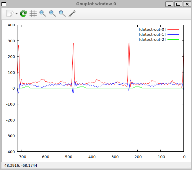
Fig. 61. The gnuplot window from running ninja ecg-detect-qrs - MIT-BIH record 205, 720 samples (2 s), RTL
In Fig. 61, three signals are visible, corresponding to the three fields of the detect_out stream:
[detect-out-0] red line - MLII centered (mlii − 900)
The raw ECG signal from lead MLII, shifted by the 900 ADC baseline point so that the zero axis corresponds to the isoline. Two sharp spikes (amplitude ≈ 280 ADC ≈ 1.4 mV) around samples 520 and 350 from the right edge represent two consecutive QRS complexes. The clear QRS morphology, with a dominant R peak, confirms the band-pass filter is working correctly - noise has been suppressed while the peak retained its amplitude.
[detect-out-1] blue line - V1 centered (v1 − 900)
The signal from lead V1 of the same recording. QRS morphology in V1 is, as a rule, less pronounced than in MLII, which is visible in the figure - the blue signal shows a smaller R-peak amplitude at similar QRS time positions. Having both channels available at once allows distinguishing supraventricular contractions (APC) from ventricular ones (PVC), since ventricular QRS complexes show a distinct morphology in V1.
[detect-out-2] green line - the QRS detection signal ((mwi − 2·mwi_thr) × 5)
The algorithm’s output signal. A positive value means a detected QRS complex - the moving-window-integration envelope exceeded twice the adaptive threshold. In the figure, two clear positive pulses are visible, coinciding in time with the QRS peaks on the MLII channel. Between beats, the line stays close to zero or slightly below - confirming the detector’s specificity.
The gap between the two visible QRS complexes is approximately 170 samples, which at 360 Hz gives:
RR ≈ 170 / 360 ≈ 0.47 s → HR ≈ 127 bpm
This value falls within the range of ventricular tachycardia (VT, 79–216 bpm) recorded in record 205, suggesting that the visualized fragment of the recording comes from one of the 6 VT episodes noted by the MIT-BIH cardiologists.
Process flow diagram
The diagram below (Fig. 62) shows the complete data flow from the raw MIT-BIH recording to arrhythmia identification, indicating where RetractorDB carries out the Pan-Tompkins algorithm, and its relationship to classic arrhythmia-recognition methods:
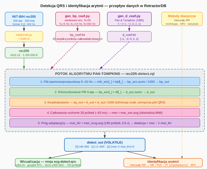
Fig. 62. Data flow - from the MIT-BIH recording, through the Pan-Tompkins pipeline in RQL, to visualization and arrhythmia identification
The right branch of the diagram - Arrhythmia identification - represents classic post-QRS-detection analysis methods, which can be built as further RQL queries layered on top of the detect_out stream:
| Method | Description | Relationship to QRS |
|---|---|---|
| RR intervals | Time between consecutive QRS complexes → HR | directly from detection positions |
| HRV (variability) | Standard deviation of RR | RR-stream statistics |
| PVC classification | QRS width > 120 ms, V1 morphology | width of the mwi window |
| VT detection | Sequence of ≥ 3 PVCs with HR > 100 bpm | RULE on the HR+PVC stream |
| APC detection | An early, narrow QRS preceding a pause | MLII vs V1 morphology |
RetractorDB provides RULE operators and windowed reducers (AVG, SUMC), which make it possible to implement the methods above in the same RQL query language, without leaving the system’s environment. QRS detection is the first and necessary step in this hierarchy.
Candlestick Chart (OHLC)
A candlestick chart is the basic way of presenting quotes in technical analysis. Each time interval is described by four values: open, high, low and close. The candle body spans from the open to the close, and the wicks reach the high and the low of the interval.
This example shows how to build candles from a regular stream using RQL queries alone, and how xqry --gnuplot-ohlc draws them on a shared axis together with the samples they were built from. The data source is random bytes, smoothed by a moving average into a trace that resembles a price. This is not market data - the example demonstrates the mechanism, not the analysis of quotes.
The RQL query
The file examples/candlestick/candlestick.rql:
STORAGE 'temp'
DEFAULT VOLATILE
DECLARE v BYTE STREAM source, 0.02 DEVICE '/dev/random'
SELECT int(AVG(source[0] : 25)) STREAM price FROM source
SELECT * STREAM bar FROM price@(10,-10)
SELECT * STREAM hi FROM MAX(bar)
SELECT * STREAM lo FROM MIN(bar)
SELECT bar[0], int(hi[0]), int(lo[0]), bar[9] STREAM ohlc FROM bar + hi + lo
SELECT * STREAM chart FROM ohlc + bar
The plan consists of the following streams:
| Stream | Interval | Fields | Role |
|---|---|---|---|
source | 0.02 s (50 Hz) | 1 | bytes read from /dev/random |
price | 0.02 s | 1 | moving average of 25 samples - the “price” |
bar | 0.2 s | 10 | tumbling window: 10 price samples in arrival order |
hi | 0.2 s | 1 | maximum of the bar record |
lo | 0.2 s | 1 | minimum of the bar record |
ohlc | 0.2 s | 4 | open, high, low, close |
chart | 0.2 s | 14 | the candle and the ten samples it was built from |
The DEFAULT VOLATILE directive keeps all results and substrates in memory, so the example persists nothing to disk (→ VOLATILE Clause). The temp directory named by STORAGE must still exist before the server starts.
The price stream comes from the record-window aggregate AVG(source[0] : 25). An aggregate in the SELECT list reduces vertically, over successive history records, so it turns white noise into a slowly varying trace, and the result interval stays equal to the source interval. The average has type RATIONAL, so the query casts it to an integer with int(...) - for the same reason as in the signal filter example: gnuplot would read only the numerator of a fraction.
The bar stream is the window price@(10,-10). The step and the width are equal, so this is a tumbling window: every price sample falls into exactly one candle, and a new record appears every 10 × 0.02 s = 0.2 s. The negative width means mirrored aggregation - the fields are ordered by arrival, so bar[0] is the oldest sample of the window (the open) and bar[9] the newest (the close) (→ Window Types).
The hi and lo streams use the MAX(bar) and MIN(bar) reducers in the FROM clause. A stream reducer folds the fields of one record horizontally, so it yields the maximum and minimum of the candle’s ten samples at an unchanged 0.2 s interval (→ Aggregate Operators). The reducer result also has type RATIONAL, hence int(hi[0]) and int(lo[0]) in the next query.
A record-window aggregate could not replace the @ window here. MAX(price[0] : 10) in the SELECT list slides by one record and emits a result every 0.02 s, so it would produce ten overlapping candles for every real one. Only the tumbling window defines the candle’s boundaries and its interval.
The sum bar + hi + lo joins three streams with the same interval into a 12-field record, from which ohlc selects the four candle values. The last query, ohlc + bar, appends the candle’s ten samples to it. The chart record therefore has 14 fields: open, high, low, close, and the samples in arrival order. Since a candle and its samples arrive in one record, the client does not need to align two separate streams in time.
The --gnuplot-ohlc mode
The --gnuplot-ohlc option is a modifier of the -p / --gnuplot mode of xqry (→ xqry). It expects a record with the layout:
open, high, low, close, sample_1, ..., sample_N
The number of samples N follows from the record length (N = number of fields - 4) and needs no separate parameter. Drawing follows these rules:
- Each record gives one candle, placed over the middle of the span occupied by its N samples. The candle body is 80% of that span wide.
- A candle whose close is not lower than its open is green (rising); the others are red (falling). The samples are drawn as a blue line.
- The first
-pparameter counts samples, as in the ordinary gnuplot mode. The window therefore holds as many candles as the window width divided by N. - The newest sample sits at x = 0. The
--gnuplot-rtlmodifier reverses the axis, so the newest candles appear on the right. - A candle in which any of the four values is
NULLis skipped entirely; its samples stay on the chart. - A record without samples (4 fields or fewer) is not drawn.
xqrythen prints a one-time message onstderr, e.g.xqry: --gnuplot-ohlc needs open, high, low, close and at least one sample; stream 'ohlc' sends 4. Standard output goes to gnuplot, so without this message the window would stay empty with no explanation. - Calling
--gnuplot-ohlcwithout--gnuplotends with the error--gnuplot-ohlc requires --gnuplot/-p mode.
Running
The candlestick target in the build system displays the chart:
# from build/Debug or build/Release
ninja candlestick
CMake runs the following invocation in the examples/candlestick directory:
scripts/xplot.sh chart candlestick.rql 250,64,192 "--gnuplot-ohlc --gnuplot-rtl"
Meaning of the parameters:
| Parameter | Meaning |
|---|---|
chart | The name of the output stream |
candlestick.rql | The query file |
250 | The window width in samples - 25 candles of 10 samples |
64,192 | The Y-axis range; the average of 25 random bytes centers on 127.5 |
--gnuplot-ohlc --gnuplot-rtl | Candlestick mode, newest candles on the right |
The scripts/xplot.sh script works the same way as in the ECG signal analysis example: it recreates the temp directory, starts a named xretractor instance in the background, and pipes the stream through xqry into gnuplot.
Without the script, the example can be run in two terminal windows from the examples/candlestick directory:
$ mkdir -p temp && xretractor candlestick.rql
$ xqry -s chart -p 250,64,192 --gnuplot-ohlc --gnuplot-rtl | gnuplot
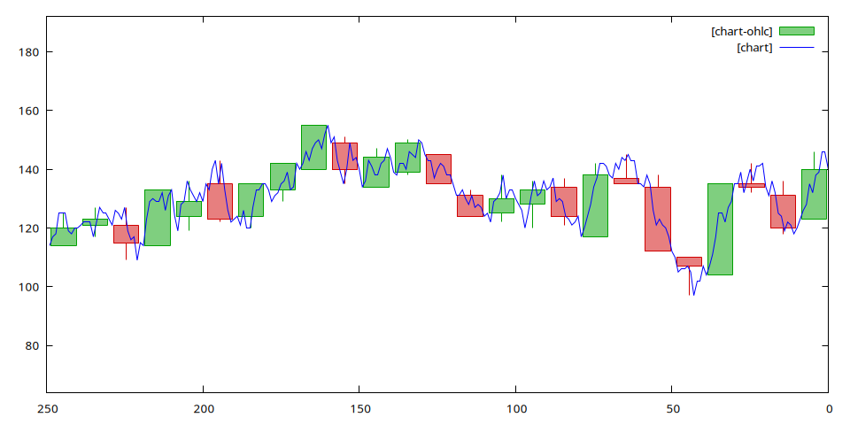
Fig. 63. Candlestick chart of the chart stream - 25 candles of 10 samples, newest on the right
Fig. 63 shows one data frame sent by xqry --gnuplot-ohlc --gnuplot-rtl and rendered by gnuplot. Each candle covers exactly ten samples of the blue line: one edge of the body lies on the first sample of the span (the open), the opposite edge on the last one (the close), and the wicks reach the highest and lowest sample of the span. The open of each candle lies close to the close of the previous one, because price is a moving average and changes smoothly across spans.
NOTE: The
--gnuplot-ohlcmode is checked by theut_formatterunit tests: candle placement over its samples, window width counted in samples, skipping a candle with aNULLvalue, and a record without samples.
Appendices
The appendices contain documents not directly related to the system’s construction, but which describe the motivation behind design decisions, tool documentation, and supporting material for people deploying or extending the system.
-
Production Builds and Diagnostic Variants
A description of the production
releasesafety contract and the isolatedrelease-ablationandprobemodes. The chapter covers source-tree cleanliness checks, explicit optimizer-switch values, separate CMake and Conan directories, verification of the resulting binary configuration, and the value-equivalence invariant across variants. -
A versioned JSON Lines contract and optional Python and C++ libraries for observing streams from an explicitly named instance. This chapter describes type mappings, subscription lifecycle, timeouts, bounded buffers, error handling, and the separate targets used to build, install, and test the API.
-
A description of the historical circumstances that led to RetractorDB’s creation. The starting point is the author’s experience building a neonatal monitoring system in the early 2000s - running into the limitations of relational databases when recording high-granularity signals, attempts based on the stream-processing systems of the time, and the evolution toward a dedicated time-series processing engine. The chapter also explains where the name “Retractor” comes from - a reference to a group of surgical instruments that separate and join tissue structures, treated here as an analogy for operations on data streams.
-
RetractorDB query files (extension
.rql) have dedicated syntax-highlighting definitions for three environments:- Visual Studio Code - the
rql-vscodeextension, installed from the GitHub repository, - Vim - the files
syntax/rql.vimandftdetect/rql.vim, installed viascripts/buildrdb.sh vimsyntaxor manually into~/.vim/, - bat / batcat - a Sublime Text 3 format definition, installed via
scripts/buildrdb.sh batsyntax.
Each environment recognizes RQL keywords (
SELECT,DECLARE,RULE,STREAM, …), data types, comments, string literals, and numeric values. - Visual Studio Code - the
-
Complete command-line flag documentation for all three of the system’s tools:
Tool Role xretractorThe main processing process: compiles RQL queries and executes the plan xqryClient: queries a running xretractorvia shared memoryxtrdbInspection tool: analyzes binary artifacts and metadata Each tool is described in its own subchapter, with example invocations and explanations of the individual switches.
-
A catalog of all the system’s integration tests, with a description of the functionality each one verifies. Integration tests run the actual binaries (
xretractor,xqry,xtrdb) and compare their results against patterns - unlike GTest unit tests, which test isolated library classes.Scenarios live in the shared
test/IntegrationTesttree. Tests that start a server receive one of sixteenRDB_NAMESPACEnamespaces and a CTest resource lock for their directory, so most can run concurrently without stream-name, IPC, or working-file collisions. Scenarios examining global identity, cooperation between multiple servers, or leftover cleanup may requireRUN_SERIAL.Running them:
ninja testorctest -R <name> -Vin thebuild/Debug/directory. -
Installing a Linux release through
curlor apt, upgrades and removal, building from source, and configuration checks. A separate section covers Apple solely as a development environment.
Production Builds and Diagnostic Variants
The scripts/buildrdb.sh script provides the production release build and diagnostic modes. The release-ablation and probe variants have separate CMake configurations, output directories, and Conan generators. Verification of the resulting binary confirms its switches. Tool preparation and installation are described in Installation Process.
⚠️ Warning
Binaries produced by
release-dirty,release-ablation, andprobeare diagnostic variants. They must not be installed or packaged as production releases.
Build modes
| Command | Purpose | Binary directory |
|---|---|---|
scripts/buildrdb.sh release | verified production release | build/Release |
scripts/buildrdb.sh release-dirty | diagnostics of local changes, without production qualification | build/Release |
scripts/buildrdb.sh release-ablation | selected optimizer and probe configuration | build/Release-Ablation/<configuration> |
scripts/buildrdb.sh probe | diagnostics with the probe enabled | build/Release-Probe |
The release-ablation and probe modes also use separate Conan generator directories:
build/Conan-Release-Ablation/<configuration>,build/Conan-Release-Probe.
Consequently, their CMake cache, compiler definitions, and binaries are not written to the production build/Release directory.
release-dirty accepts uncommitted changes and rebuilds the same build/Release directory used by release. It still sets the optimizer switches explicitly and checks --build-info, but the result is for diagnosing changes before a commit. It is neither an isolated variant nor a production release; run release again from a clean tree before preparing a release.
The production release contract
The command:
scripts/buildrdb.sh release
operates in a fail-closed mode: every failed check stops the build. The script:
- requires a Git repository and a completely clean working tree;
- rejects tracked changes, staged changes, and untracked files;
- removes the previous
build/Releasedirectory; - removes common variables that can inject compiler, linker, or CMake flags from the configuration process;
- explicitly passes the complete production configuration;
- builds the binary in a fresh directory;
- reads the configuration from the resulting
xretractor; - checks the source tree again after the build.
Variables removed from the build process environment include CFLAGS, CPPFLAGS, CXXFLAGS, LDFLAGS, CMAKE_ARGS, CMAKE_GENERATOR, and CMAKE_TOOLCHAIN_FILE. The probe runtime variables RDB_BENCH_CSV and RDB_BENCH_PLAN are not passed either.
The production configuration is always:
RDB_OPT_DEDUP_SUBSTRATES=ON
RDB_OPT_SHARE_EQUIVALENT_SELECTS=ON
RDB_OPT_COMMUTATIVE_ADD=ON
RDB_OPT_FACTOR_MATCHED_HASH_TIMEMOVES=ON
RDB_BENCH_PROBE=OFF
RDB_OPT_SIMPLIFY_EXPRESSIONS=ON
After compilation, the script runs:
build/Release/src/retractor/xretractor --build-info
and compares the result with the set above. A missing binary or any different value causes release to fail.
ℹ️ Info
The Git cleanliness check proves that the build does not use local, uncommitted changes. It does not prove that the contents of a committed revision are correct. Review, tests, and CI are responsible for that part.
Variants with disabled optimizations
The command:
scripts/buildrdb.sh release-ablation
opens a submenu that independently toggles:
RDB_OPT_DEDUP_SUBSTRATES
RDB_OPT_SHARE_EQUIVALENT_SELECTS
RDB_OPT_COMMUTATIVE_ADD
RDB_OPT_FACTOR_MATCHED_HASH_TIMEMOVES
RDB_BENCH_PROBE
RDB_OPT_SIMPLIFY_EXPRESSIONS
Each variant receives a directory that describes its complete configuration, for example:
build/Release-Ablation/dedup-OFF_share-ON_comm-ON_factor-ON_probe-OFF_simplify-ON
All six values are passed explicitly. This prevents values stored by an earlier configuration in CMakeCache.txt from being inherited.
The configuration:
RDB_OPT_SHARE_EQUIVALENT_SELECTS=OFF
RDB_OPT_COMMUTATIVE_ADD=ON
is invalid. Commutative-add canonicalization is part of equivalent SELECT computation sharing, so both the submenu and CMake reject this combination.
After building a variant, the script compares --build-info with the values selected in the submenu. A mismatch is a configuration error.
Diagnostic probe
RDB_BENCH_PROBE is optional instrumentation rather than a plan optimization. The command:
scripts/buildrdb.sh probe
builds a variant with all optimizations enabled and:
RDB_BENCH_PROBE=ON
The binary is written to build/Release-Probe. It is built from optimized Release code, but the resulting binary is not a production build.
In release-ablation, the probe can be enabled or disabled independently of a valid optimizer configuration.
The probe does not participate in the selection or order of optimizer passes. It is not zero-cost instrumentation, however: RDB_BENCH_PLAN additionally traverses the plan and writes statistics, while RDB_BENCH_CSV performs clock measurements and file operations. The probe is therefore semantically non-invasive, but its overhead can affect measured timings.
When the binary has RDB_BENCH_PROBE=ON and RDB_BENCH_PLAN is set during compilation, the compiler writes the following stable line to standard error:
REWRITE_APPLIED r1=<count> r2=<count> r3=<count>
The counters are reset before every compiler invocation. r1 is the number of successful (A > i) # (B > k) -> (A # B) > (i + k) rewrites. r2 is the number of unique STREAM_ADD nodes for which the canonical plan fingerprint actually swapped the children. r3 is the number of simplifications in field programs and RULE conditions: constant folds, combined constant tails, removed neutral elements, and replacements of a repeated exact factor by a power (E*E*E -> E^3). That last rule covers only the BYTE, INTEGER, UINT, and RATIONAL types; it does not rewrite FLOAT or DOUBLE multiplication. The counters describe applied rewrites, not speedup. With RDB_BENCH_PROBE=OFF, the counter code is absent from the binary and no REWRITE_APPLIED line is emitted.
Inspecting a variant manually
Every xretractor provides:
path/to/xretractor --build-info
The command prints the configuration and exits without starting the engine (-b is an equivalent shorthand). It is handled before the configuration file is loaded and validated, so it yields a correct result even when the host configuration would prevent the program from starting normally. An example production result is:
RDB_OPT_DEDUP_SUBSTRATES=ON
RDB_OPT_SHARE_EQUIVALENT_SELECTS=ON
RDB_OPT_COMMUTATIVE_ADD=ON
RDB_OPT_FACTOR_MATCHED_HASH_TIMEMOVES=ON
RDB_BENCH_PROBE=OFF
RDB_OPT_SIMPLIFY_EXPRESSIONS=ON
The directory name is only a convenience; the information read from the binary is the final confirmation of the compiler definitions used.
Variant tests
Disabling an optimization can intentionally change plan structure and the availability of tests that require a particular shape. It must not change the value part of the result: interval, logical origin, public descriptor, records with null maps, or materialization policy. The startup tail has the weaker guarantee described below.
CTest assigns requires_* labels to tests that need a specific optimization and can disable them for an incompatible configuration. The expected_ablation_failure label then describes the expected unavailability of a plan-shape test, not permission for semantic divergence.
Use the following procedure to assess a failure:
- run the same test in the production configuration;
- confirm that it passes with the required optimizations;
- run it in the variant being studied;
- demonstrate that the failure is caused by the disabled switch;
- if the test requires the disabled pass, disable it for that variant;
- treat every other failure as a regression.
The it_optimizer_ablation-build-info test verifies that the information reported by the binary matches the CMake configuration. The other it_optimizer_ablation-* tests check plan structures and semantic comparisons between variants.
A variant with an optimization disabled may change plan structure, but it must not change values, NULL maps, the public descriptor, logical origin, or materialization policy. A correct plan rewrite may shorten the tail, but it must not cause emission before the data is available. Any other divergence is a regression, not an admissible property of a variant.
Packaging
Prepare production packages only after a successful, verified release:
scripts/buildrdb.sh release package
The package option restores the production switch values and rebuilds the selected directory before running CPack. Do not run packaging from Release-Ablation or Release-Probe directories.
Packages serve different purposes:
| Variant | Default contents and paths |
|---|---|
Linux: package (DEB/TGZ) | Three programs under /usr/bin, a systemd unit, license, default TOML, and configuration examples. |
Linux: package-portable | Relative paths: bin/, share/doc/retractordb/LICENSE, share/retractordb/retractor.toml; no systemd unit. The web installer can create the service. |
Apple development port: package (TGZ) | /usr/local prefix, without the systemd service component; no launchd configuration is supplied. |
CPack does not generate a source package. The it_packaging test checks the exact contents of the DEB when dpkg-deb is available, and of the portable archive. Scripts for preparing Linux release assets live in scripts/release_package/; running them and publishing assets are separate from local installation.
Platform capabilities and sanitizers
CMake configuration checks the available platform functions and records RDB_HAS_* results in generated/platformConfig.h. The RDB_PLATFORM_FALLBACKS list specifies deliberately allowed fallback paths. It is empty by default on Linux. If a controlled probe selects an undeclared fallback, configuration fails; inspect CMakeFiles/CMakeConfigureLog.yaml before adding a missing function to the list.
The CMake option -DRDB_SANITIZE=address,undefined enables AddressSanitizer and UndefinedBehaviorSanitizer; detected undefined behavior terminates execution. This is a CMake configuration argument, not an additional buildrdb.sh option. Sanitizers require rebuilding the binaries under test.
On the Apple development port, the ready-made entry point is scripts/macos-build.sh --sanitize. Running ordinary tests without Valgrind does not enable sanitizers automatically. scripts/macos-build.sh release selects the Release configuration but does not implement the production contract of buildrdb.sh release. See Apple development environment for the full workflow and limitations.
Optional client API
The api/ directory is developed and tested with the engine, but it is not part of the default product. Plain ninja, ninja install, ninja test, and ninja package leave the API libraries and tests out of their results.
The explicit entry points are separate:
| Command | Meaning |
|---|---|
ninja install-withapi | Builds and installs the engine and the api component. |
ninja test-api | Builds the C++ test client and runs tests carrying the api label. |
cmake -DRDB_WITH_API=ON . | Adds the api component to CPack packages; the ordinary test target then stops filtering out the api label. |
The packaging switch must be set during configuration because CPack determines its component list at that point. Without RDB_WITH_API=ON, packages contain no API libraries; their remaining contents depend on the package variant described above. The it_packaging test protects the default Linux DEB and portable contents.
C++ API targets are always known to CMake, but use EXCLUDE_FROM_ALL. Their installation rules belong to the separate api component, so ninja install alone does not run them. Library usage and the JSONL contract are described in Stream Monitoring API.
Stream Monitoring API
The optional client API monitors streams from a running, explicitly named xretractor instance on the same Linux host. Its transport layer starts xqry --jsonl processes, so the API does not duplicate the Boost IPC protocol and follows the command-line tool’s rules for selecting streams and ending subscriptions.
The following interfaces are available:
- a Python 3.10+ package with no runtime dependencies beyond the standard library;
- a static C++23 library with a public header and CMake configuration;
- a versioned JSON Lines v1 contract that can also be consumed without either library.
The API does not start the server, load plans, reconnect after failure, or replay missed samples. It is a live observation interface, not a durable or lossless transport.
JSON Lines v1 contract
xqry --jsonl supports four read-only commands:
xqry --server laboratory --jsonl --hello
xqry --server laboratory --jsonl --dir
xqry --server laboratory --jsonl --detail temperature
xqry --server laboratory --jsonl --select temperature --elimitqry 10
Every stdout line is a complete UTF-8 JSON object with version: 1 and an event field. Diagnostic messages go to stderr.
| Event | Contents |
|---|---|
pong | Response to hello. |
streams | An array of {name, delta} items; empty for an idle server. |
schema | Stream name, interval, original query, and ordered fields. |
record | Stream name and a flattened value array. |
end | Normal completion: limit or server_stopped_or_reloaded. |
error | Stable error code and description; the process exits non-zero. |
A subscription emits its schema first, then records, and exactly one final end or error event. EOF without a final event is a process error even when the exit code is zero.
{"version":1,"event":"schema","stream":"temperature","delta":"1/20","query":"...","fields":[{"name":"v","type":"INTEGER","count":2}]}
{"version":1,"event":"record","stream":"temperature","values":["21",null]}
{"version":1,"event":"end","reason":"limit"}
The schema’s count field is the scalar cardinality. Numeric arrays preserve every element and its individual NULL value; STRING[N] remains one string. Non-null wire values are strings interpreted according to the schema type. This preserves rational numerators and denominators and distinguishes the string "null" from JSON null.
| RQL type | Python | C++ Value |
|---|---|---|
NULL | None | std::monostate |
BYTE, INTEGER, UINT | int | std::int64_t |
FLOAT, DOUBLE | float | double |
RATIONAL | fractions.Fraction | Rational |
INTPAIR | pair of integers | std::pair<int64_t, int64_t> |
IDXPAIR | string-integer pair | std::pair<std::string, int64_t> |
STRING | str | std::string |
Messages carry neither a source timestamp nor a durable sequence number. Floating-point precision is limited by the existing textual IPC serialization, and the complete INFO wrapper must fit the server queue’s 1024-byte limit.
--idle-timeout N ends JSONL after N milliseconds without a record; zero disables the limit. This is independent of the per-read timeout exposed by the libraries.
Python
Install the package from source:
python3 -m venv .venv-api
.venv-api/bin/python -m pip install ./api/python
Every subscription owns a child xqry process:
from retractordb import Client, ReadTimeout
with Client("laboratory", xqry="/path/to/xqry") as db:
print(db.streams())
print(db.describe("temperature"))
with db.subscribe("temperature", limit=10) as samples:
for record in samples:
print(record["v"])
print(samples.end_reason)
Client(server, xqry="xqry", timeout=5.0) accepts a timeout in seconds. subscribe(stream, limit=0, idle_timeout=0.0, capacity=1024) returns an object whose schema is already known when the call returns. next(timeout=...) may raise ReadTimeout without closing the subscription; ordinary iteration waits indefinitely. A record maps each field name to a scalar or an array of elements.
Use context managers or call close() explicitly. Merely breaking out of a for loop does not close the iterator. The library does not install signal handlers for the application.
ping() returns True after a valid server response; on failure it raises Error with the error code and cause description. It does not return False or hide transport or protocol failures. Example error handling:
from retractordb import Client, Error
with Client("laboratory", xqry="/path/to/xqry") as db:
try:
db.ping()
except Error as exc:
print(f"Ping failed: {exc.code}: {exc}")
else:
print("Server responded")
Python compatibility: the True result preserves the behavior of existing if db.ping(): and assert db.ping() code. Both calls raise an exception on failure. The contract approved in #425 preserves the success result in Python; C++ uses void.
C++
The library requires C++23. Its targets are available on demand in the RetractorDB tree:
cmake --build build/Debug --target rdb_monitor
build/Debug/api/cpp/rdb_monitor laboratory temperature 10 /path/to/xqry
A project may include the sources directly:
add_subdirectory(/path/to/retractordb/api/cpp rdb-api)
target_link_libraries(my_monitor PRIVATE RetractorDB::client)
After installing the API component, a CMake package is available:
find_package(RetractorDBClient CONFIG REQUIRED)
target_link_libraries(my_monitor PRIVATE RetractorDB::client)
Minimal subscription:
#include <iostream>
#include "retractordb/client.hpp"
int main() {
retractordb::Client db("laboratory");
auto samples = db.subscribe("temperature", {.limit = 10});
while (auto record = samples.next())
std::cout << record->values.at("v").size() << '\n';
}
SubscribeOptions exposes limit, idleTimeout, and capacity. next(timeout) returns std::optional<Record>; an empty value means normal completion or an explicit close. Errors throw retractordb::Error with a stable code field. Subscription handles are movable but not copyable; the destructor and close() terminate and reap their child process.
Client is also movable and noncopyable. Its move constructor and move assignment are noexcept and defined = default outside the header. Moving transfers ownership of the client and its subscriptions; move assignment first closes the destination’s previous subscriptions. The client destructor closes its subscriptions even if their handles still exist. The accessors Client::streams(), describe(), and subscribe(), and Subscription::schema(), next(), pid(), and endReason() are [[nodiscard]].
Client::ping() returns void after a valid response and throws retractordb::Error with the error code and cause description on failure. Successful completion without an exception indicates success; there is no false result.
Moved-from client: the source Client can safely be destroyed, closed with close(), or assigned another client. Calls to ping(), streams(), describe(), and subscribe() throw retractordb::Error with code closed. Assigning a working client makes the object usable again. After an ordinary close(), these methods also report closed when called with valid arguments.
Limits and error handling
Library buffers are bounded: by default, 1024 pending events, 1 MiB per JSONL line, and 64 KiB of retained stderr. An application-buffer overflow produces buffer_overflow and closes the subscription without silently dropping records. A server-side queue overflow is a limitation of the existing IPC and may surface only as an idle timeout.
Closing is idempotent: the library sends SIGTERM to its own xqry, waits for up to one second, then uses SIGKILL if necessary and reaps the process. Closing a client closes all of its subscriptions; it never sends xqry --kill to the server.
Error codes include read_timeout, idle_timeout, buffer_overflow, stream_not_found, no_active_plan, server_stopping, server_no_response, client_queue_missing, disconnected, communication_error, protocol_error, spawn_error, process_exit, process_timeout, and closed.
Building and testing
The API is developed with the engine but remains optional. Plain ninja, ninja install, ninja test, and ninja package do not build, install, test, or package the API.
| Command | Effect |
|---|---|
ninja install-withapi | Builds and installs the engine and the api component. |
ninja test-api | Builds the test client and runs ctest -L api. |
cmake -DRDB_WITH_API=ON . | Adds the api component to CPack packages and API tests to the ordinary test target. |
The C++ API is always configured, but its targets use EXCLUDE_FROM_ALL. xqry has its own Boost.JSON translation unit, so the engine does not link anything from api/. The dependency runs only from the API to the public xqry process interface.
The st_api_fake and st_api_real tests cover both languages. The former covers types, NULL, malformed output, overflow, and process cleanup. The latter uses a real xretractor and checks independent subscriptions, arrays, rational numbers, a missing stream, and server shutdown.
The C++ tests also cover a client factory, std::vector, lambda capture, move assignment with active subscriptions, and safe close() and destruction of a moved-from object. They check the closed code from all four client methods after move construction, move assignment, and explicit closure. Both languages check successful and failed ping() calls and preservation of the protocol_error, server_no_response, and closed codes; the Python tests require a True result on success.
Command-Line Options
RetractorDB consists of three command-line tools, each playing a distinct role in the system’s architecture:
| Tool | Role |
|---|---|
xretractor | Processing process: compiles RQL and executes one independent plan |
xqry | Client: discovers or selects an instance and communicates through its IPC |
xtrdb | Inspection tool: analyzes binary artifacts and metadata |
Each tool is described in its own subchapter.
xretractor
The xretractor program is RetractorDB’s core process. It compiles files containing RQL queries and executes the data-processing plan. It’s built to run autonomously as a systemd daemon process.
Modes of operation
xretractor starts in one of two modes:
| Mode | Description |
|---|---|
| Processing | Default - compiles queries and starts the query-execution loop |
Compile only -c | Compiles queries without starting the loop; allows visualizing the plan |
Calling -h shows a different option list depending on the mode - option shorthands overlap, so pay attention to which mode a given option applies in.
Processing mode (default)
$ xretractor -h
xretractor - compiler & data processing tool.
Usage: xretractor queryfile [option]
Available options:
-h [ --help ] Show program options
-b [ --build-info ] show optimizer build configuration
-c [ --onlycompile ] compile only mode
-q [ --queryfile ] arg query set file
-r [ --quiet ] no output on screen, skip presenter
-s [ --status ] check service status
-o [ --cleanup ] remove leftovers of dead instances and exit
-v [ --verbose ] verbose mode (show stream params)
-x [ --xqrywait ] wait with processing for first query
-n [ --name ] arg instance name; own IPC area and lock
-a [ --autoname ] generate a docker-style instance name
-k [ --noanykey ] do not wait for any key to terminate
-j [ --service ] service mode: log to stderr (journald)
-t [ --realtime ] enable real-time scheduling
-f [ --no-clock ] offline mode: compute slots without waiting
-u [ --until-eof ] forces one-shot all sources
-g [ --config ] arg config file (TOML); overrides search
-m [ --llimitqry ] arg (=0) loop iteration limit, 0 - no limit
Processing-mode options
| Option | Meaning |
|---|---|
help | Displays the help text. The list differs depending on the mode (with or without -c). |
build-info | Prints the optimizer configuration the binary was built with (the RDB_OPT_* flags and RDB_BENCH_PROBE) and exits without starting the engine. It is handled before the configuration file is loaded and validated, so it also works on a host with an invalid storage.dir. The output is stable and meant for automated processing - both scripts/buildrdb.sh and the it_optimizer_ablation-build-info test rely on it. See the appendix on production builds and diagnostic variants for details. |
onlycompile | Switches the tool into “compile only” mode. The query-execution loop is not started. |
queryfile | The name of the query file to compile and run. |
quiet | Skips displaying results on screen. Processing runs normally, but the result presenter isn’t started. |
status | Checks the instance lock selected by --name, RDB_NAMESPACE, or the historical empty name. Running means another process holds the same identity. |
cleanup | Removes recognized leftovers of dead instances and exits without starting a plan. Also available as -o. Live owners remain protected; scope and limitations are described below. |
verbose | Shows stream parameters and adds on stderr a message about streams growing without bound on disk and warnings about declarations in the deprecated DECLARE ... FILE form (one per declaration, with the plan line and the chosen keyword BINFILE, TEXTFILE or DEVICE). Without this option there are no warnings about the deprecated form. A separate log entry depends on the logging level. |
xqrywait | Compiles the queries and holds off the processing loop until the first client command has been handled. When receiving data through xqry from a run limited by -m N, it prevents the entire budget from being processed before the client connects. xqry --select registers its subscription first, so its queue exists before the loop is unblocked. However, any handled command releases the gate, including --hello or --dir from another client; this does not mean all receivers are ready. A stop signal interrupts the wait without executing the zero step. When inspecting files after the run has finished, -x is not needed. |
name arg | Gives the instance a stable name. The name selects a separate lock file and IPC area and lets commands be routed through xqry --server. It may contain at most 32 lowercase letters, digits, _, and -, and its first character must be a letter. |
autoname | Generates a container-style instance name and prints it at startup. Mutually exclusive with --name. |
noanykey | Disables stopping the processing loop on any keypress. A positive --llimitqry N limit also disables this behavior, even without --noanykey. A keypress stops an unlimited run if this option was not supplied. Ctrl+C still stops the process. |
service | Service mode: the log goes to stderr (captured by journald), with no log file in the temporary directory, no timestamp of its own, and no ANSI codes. The mode can also be enabled through the XRETRACTOR_SERVICE environment variable set to any value other than empty or 0 - convenient in a systemd unit via Environment=. |
realtime | Enables real-time scheduling of the processing thread: SCHED_FIFO, mlockall, and moving the communication thread off the cores assigned to the processing thread. It does not change the slot schedule: sleeping until a deadline counted from a fixed anchor applies in every clocked mode (see Slot schedule). Requires CAP_SYS_NICE and CAP_IPC_LOCK capabilities (or root); without them it prints the compliance report and runs without these settings. Recommended in production environments requiring deterministic response time. |
no-clock | Offline mode: retains the rational timeline, logical indices, origins, and plan tails, but skips wall-clock waiting. The TIMEOUT deadline of every DEVICE source is then 0. It cannot be combined with --realtime. |
until-eof | Switches declared sources to ONESHOT mode and stops when the first one runs out of data. For a DEVICE source exhaustion is the first end of data after data was received, that is, the writer leaving. |
config | Path to a configuration file in TOML format. It overrides the standard search order (/etc/retractor/retractor.toml, then $XDG_CONFIG_HOME/retractor/retractor.toml or ~/.config/retractor/retractor.toml). Missing files at those locations allow built-in defaults to be used; a missing file explicitly selected with --config is an error. |
llimitqry | Limits the number of iterations in the query-execution loop. A value of 0 means no limit. |
Multiple instances
Several named instances can run concurrently:
xretractor measurements.rql --name measurements --noanykey &
xretractor diagnostics.rql --name diagnostics --noanykey &
xqry --bus
Each receives its own lock and IPC objects. The shared bus nevertheless rejects a plan that collides with a live instance by stream name, written storage file, or :ROTATION counter file. The check happens before artifacts are removed. Omitting --name preserves the historical unnamed instance.
Service mode provides a separate guarantee: exactly one service instance may run in each RDB_NAMESPACE; in the default namespace it is named service. See Multiple Instances and the Bus.
The instance lock file must be a regular file with a single name, owned by the account that starts the instance. A symbolic link (dangling ones included), a second hard link, a directory or a FIFO at that path, as well as a file owned by another account - also for an instance started as root - stop startup without changing the contents of the target file. The stderr message, shown in Release builds as well, names the path and the cause, and exit code 5 (EIO) distinguishes this refusal from an identity that is already taken (37, ENOLCK, message is already running). A leftover of another account after a crash is neither taken over by the instance nor removed by --cleanup; an operator with rights to the lock directory removes it by hand. Reading presence and IPC identity locks of other accounts remains allowed.
Cleaning up leftovers
xretractor --cleanup
The command does not start a plan. It attempts to acquire locks on recognized resources and removes only those without a live owner holding the lock. The same mechanism runs when an instance exits.
| Scope | Action |
|---|---|
| Instance lock files | Scans paths.lock_dir selected by configuration, defaulting to the process’s temporary directory. |
| IPC identities | Scans the shared /tmp; removes an abandoned lock and its command queue, response segment, and map mutex. |
| Bus | Removes unused segments of the current xrdbbus_v7 layout protected by presence locks. |
The scope is not restricted to an instance selected with --name or a single RDB_NAMESPACE. Filesystem permissions still control access to resources. The command does not enumerate or remove client response queues; it also leaves v5 and older segments untouched because they do not participate in the presence-lock protocol.
The output counts removed instance locks, IPC identity sets, and segments, for example:
Removed leftovers of dead instances: 1 instance lock(s), 1 IPC identity set(s), 1 bus segment(s).
The IPC-set count is not a count of individual queues. Completion does not establish that resources outside the command’s scope were removed. For a custom lock directory, select the appropriate TOML using --config.
Clock-free batch processing
The simplest run over a complete input file without manually selecting an iteration count is:
xretractor query.rql --no-clock --until-eof --noanykey --quiet
--no-clock removes sleeps only. It does not change slot order or artifact content, making it suitable for fast verification after completion. It can outrun an xqry client, however, so it is not intended for live observation.
--until-eof prevents a sequential source from returning to the start of its file. EOF is checked after a slot has been processed, exactly before the first record that would otherwise have to use synthetic NULL beyond the input. A DEVICE source is read at the start of the slot, so its exhaustion is checked before the slot - with the same effect. With several sources, the first exhausted one stops the run so the plan does not continue with a missing input. It may be combined with -m N; whichever condition occurs first wins.
⚠️ Warning Short options depend on the mode. During execution,
-fmeans--no-clockand-umeans--until-eof. With-c, the same letters mean--fieldsand--rules, respectively, and do not start processing.
NOTE:
noclock_offlineverifies equivalence between paced and offline execution;untileof_stopverifies first-EOF termination and the non-wrapping control.
Compile-only mode (-c)
$ xretractor -h -c
xretractor - compiler & data processing tool.
Usage: xretractor -c queryfile [option]
Available options:
-h [ --help ] show help options
-b [ --build-info ] show optimizer build configuration
-c [ --onlycompile ] compile only mode
-q [ --queryfile ] arg query set file
-r [ --quiet ] no output on screen, skip presenter
-v [ --verbose ] verbose mode (show stream params)
-d [ --dot ] create dot output
-m [ --csv ] create csv output
-f [ --fields ] show fields in dot file
-t [ --tags ] show tags in dot file
-s [ --streamprogs ] show stream programs in dot file
-u [ --rules ] show rules in dot file
-i [ --hideruleprog ] hide rule program in rules (-u) output
-p [ --transparent ] make dot background transparent
-w [ --diagram ] arg create diagram output
-z [ --shmbudget ] show shared memory budget of the compiled plan
-g [ --config ] arg config file (TOML); overrides search
In this mode, options for creating diagrams and diagnostic dumps, described in more detail elsewhere in this work, are available. -v is also available when compiling without running the plan.
Visualization and diagnostic options
| Option | Meaning |
|---|---|
help | Displays the help text (identical to processing mode; the list differs depending on the mode). |
build-info | Identical in meaning to processing mode - prints the optimizer configuration and exits. The -c flag does not affect the output; the option is available in both modes so that the configuration dump can be obtained regardless of how the program is invoked. |
onlycompile | On - this table describes the options that apply while the -c flag is active. |
queryfile | The name of the query file to compile. |
quiet | Tests only the compilation process itself, without presenting results. The other presentation options are not started. Included for development purposes. |
dot | Creates a text file in DOT format describing the hierarchical structures produced by the compiler. The file can be passed to the Graphviz tool to generate a graphical description of the dependencies. |
csv | Exports the hierarchical data structures to a CSV file (comma-separated values). |
fields | Adds, to the DOT graph, the fields and their types for each data stream. |
tags | Adds, to the DOT graph, the internal-language programs that build the fields of each query. Must be called together with fields - it visually links the fields to their programs. |
streamprogs | Adds, to the DOT graph, the stream-algebra programs that build each query’s streams. |
rules | Adds alerting rules to the graph. |
hideruleprog | Hides the programs describing the alerting conditions (used together with rules). |
transparent | Generates the graph with a transparent background. |
diagram | Generates marble diagrams. The argument takes the form type:cycle_count: type (0 or 1) determines whether the diagrams show timestamps; cycle_count sets the number of cycles shown in the diagram. |
shmbudget | Reports the fixed IPC reservation, capacity, and free space of the shm_open filesystem (usually /dev/shm), plus the cost of one client queue for each plan interval. This lets an operator estimate the number of concurrent subscriptions before starting a server. |
config | Selects an explicit TOML file in -c mode as well; retention and history budget settings apply during compilation. |
Configuration file (TOML)
The --config option (short form -g) points at a configuration file, including in -c mode; without it the program searches two locations in layered fashion, in the order given, each later layer overriding keys from the previous one:
/etc/retractor/retractor.toml- system layer,$XDG_CONFIG_HOME/retractor/retractor.toml(or~/.config/retractor/retractor.toml) - user layer.
The absence of discovered files is a valid state - the program starts with default values. An existing file with invalid TOML stops startup: the program returns a nonzero exit code and reports an ERROR diagnostic naming the file and cause, including in Release builds. Every loaded layer must be valid, even if a later layer would override its keys. With an explicit path (--config), a missing file remains an error as well. The same configuration loader is used by xqry (--config, short option -e) and xtrdb; these programs also refuse to run with a malformed file. The --help option works in all three programs regardless of the configuration; xretractor then reports the error in the Config: line of its help. The [ipc] and [timing] sections apply to the engine and the xqry client.
| Key | Default | Meaning |
|---|---|---|
storage.dir | (none) | Default artifact directory. Applied only when the RQL set contains no :STORAGE directive - RQL wins. The directory must exist and be writable, otherwise the program exits with Configuration error: storage.dir …. |
storage.default_retention | (none) | Pair [capacity, segments], both positive. Sets bounded retention on DEFAULT and DIRECT file streams without their own RETENTION, including substrates. It does not change MEMORY, stores without retention, or explicit retention. An invalid value logs a warning and leaves default retention unset. |
storage.ref_dirs | (none) | Read by xtrdb. A list of absolute paths to existing directories where the REF field of a retained .desc may relocate a writable data file. Without this key, a REF taken from .desc permits writing and deletion only within the storage directory; reading BINFILE, TEXTFILE, and DEVICE sources and using a REF from the plan are unrestricted. In xretractor, the REF of a retained .desc must equal the plan’s REF, so this key does not change engine behavior. An invalid entry stops xtrdb at startup with Configuration error: storage.ref_dirs .... |
sources.timeout_s | (none, i.e. 0) | Read deadline in seconds for DEVICE sources without a TIMEOUT clause (→ Reading a DEVICE source and TIMEOUT). An explicit clause in RQL wins, including TIMEOUT 0. In --no-clock mode the deadline is 0. It does not change BINFILE, TEXTFILE or timing.query_no_data_timeout_ms. A negative, non-numeric value or one above 86400 stops the start with Configuration error: sources.timeout_s …. |
ipc.queue_buffer_seconds | 10 | IPC queue depth expressed in seconds of stream; the element count is seconds / interval. |
ipc.min_queue_elements | 100 | Lower bound on queue capacity, independent of the stream interval. |
ipc.client_response_max_fails | 300 | Multiplier for the xqry response time budget. A monotonic-clock deadline is set to this value times the polling interval (10 ms) and covers both waiting for space in the command queue and waiting for the response. |
timing.server_startup_wait_s | 30 | Maximum time xqry --wait-server waits for server readiness. |
timing.server_startup_poll_ms | 100 | Polling interval while waiting for the server to start. |
timing.query_no_data_timeout_ms | 10000 | No-data timeout after which the xqry client considers the server dead. |
scheduling.rt_priority | 50 | SCHED_FIFO priority in --realtime mode; allowed range 1–99. |
paths.lock_dir | (system temp directory) | Directory for instance lock files. For systemd services, /var/run/retractor or $XDG_RUNTIME_DIR is recommended. A nonempty path must be absolute in every loaded layer; a relative path stops startup with an ERROR diagnostic naming the file and cause, including in Release. An empty value keeps the default temporary directory. It does not change the fixed /tmp directory for IPC identity locks. |
server.autoname | false | Generates a name when neither --name nor --autoname was given. An explicit --name wins. false preserves the historical unnamed instance. |
service.query_file | (value from the build configuration) | The query file overwritten when a set is handed to a running service. Used only as a fallback, when the service did not report its own QUERYFILE in the lock file. It must match the ExecStart argument of the systemd unit - configuration does not change ExecStart. |
service.unrestricted | false | Allows a DO SYSTEM rule in a plan accepted over the xqry --reset channel. The default value refuses such a plan as a whole (→ xqry). With true the instance leaves a warning in the log at every start, and anyone able to open its IPC objects runs shell commands under its account. The key is read at process start-up, so it is set by the same authority that writes the service’s plan file; it never opens the ad-hoc channel. |
limits.history_memory_mib | 1024 | Combined history budget for DECLARE sources and MEMORY stores in MiB. Exceeding it rejects the plan at startup, in -c, ad hoc, and during --reset. It must be positive; an invalid value logs a warning and restores the default. See Plan Size Limits. |
IPC objects created by the server - the response segment, command queue, subscription queues, and bus segment - receive an explicit 0600 mode. Queue and response-segment creation uses create_only; opening an existing object requires its owner to match the process’s effective UID and its mode to be 0600. xqry must therefore run with the same effective UID as the server, including when invoked by an administrator, for example through sudo -u retractor xqry --server service --dir. Foreign objects are rejected and are not removed during cleanup. See the IPC access boundary for collision, restart, and bus behavior.
Out-of-range values do not stop the service: the program logs a warning and uses the default. The exceptions are storage.dir, whose invalidity would mean results landing somewhere unintended, or nowhere, and sources.timeout_s, whose silent replacement with the default would change how sources are waited for - both are hard errors of xretractor. xqry does not check sources.timeout_s. An invalid storage.ref_dirs is also a hard error, but for xtrdb: the list of permitted write locations must not be guessed.
Example file:
[storage]
dir = "/var/lib/retractor"
default_retention = [1000, 4]
[sources]
timeout_s = 0.01
[limits]
history_memory_mib = 1024
[ipc]
queue_buffer_seconds = 30
[scheduling]
rt_priority = 60
[paths]
lock_dir = "/var/run/retractor"
[server]
autoname = false
NOTE: Layer loading and validation are covered by the
ut_appConfigunit test; hard rejection of an invalidstorage.dir, a malformed TOML file and a relativepaths.lock_dirby theconfig_storage_validationintegration test, and the precedence and rejection ofsources.timeout_sby thedevice_timeoutintegration test.
Service and plan replacement
Starting without an .rql file, or with an empty one, creates an idle instance with working IPC. The first or a later complete plan can be loaded without restarting:
xqry --server service --reset plan.rql
The server parses and compiles the complete contents, checks retained .desc files, storage compatibility under :ROTATION, and resource collisions, reserves the new set, and then switches plans at a slot boundary. A malformed, empty, or incompatible descriptor causes a refusal with a reason; the old plan and the service startup file remain unchanged. An empty reset file returns the server to idle. On a service instance, accepted contents are also written to the service’s startup file.
The alternative xretractor new-plan.rql path detects a running systemd unit and validates the set, retained stores, and descriptors before atomically overwriting its startup file and requesting a restart. A refusal returns code 71 with nothing was changed; the running service keeps its plan. Explicitly selecting another identity with --name or --autoname starts a separate instance instead.
On a normal start, a bad .desc produces a diagnostic naming the file; a syntax error also identifies the line and column. The plan is refused before processing starts. Existing descriptors of DECLARE sources are always checked; descriptors of SELECT outputs and substrates are checked when :ROTATION preserves their files. In a systemd unit, refusing a plan before startup because of parsing, compilation, an incompatible retained store, or a bad .desc clears the service query file. The next unit start enters idle mode instead of retrying that plan; a critical FatalError clears the file as well. Outside a unit, the operator’s .rql file is left untouched. Compile-only mode (-c) neither reads retained .desc files nor clears the query file, even inside a unit.
Version Information
At the end of every help message, a line with build information is displayed:
Branch: issue_31-doc:2707ce0,
Code compiler: GNU Ver. 13.3.0,
Build time: 2512211449,
Type: Debug
| Field | Meaning |
|---|---|
Branch | The repository branch name and the commit hash the program was built from |
Code compiler | The GCC compiler version used for the build |
Build time | The compilation date and time, in YYMMDDHHMM format (here: December 21, 2025, 14:49) |
Type | The build type: Debug or Release |
The next line indicates the log file location:
Log: /tmp/xretractor.log
The file /tmp/xretractor.log records the history of invocations and the system’s internal events. In a production environment, this file should be cleaned up or rotated regularly.
The Config: Defaults line means that no TOML files were loaded. If configuration was loaded, Config: lists the file paths in load order. For a syntax error in a plan loaded from a file, the parser’s log entry also includes that file’s path.
The last line contains MIT license information, which allows safe use of the code in corporate applications.
xqry
The xqry program communicates with a running xretractor process through Boost IPC. It reads current records, displays plans and schemas, attaches individual RQL statements, replaces a complete plan, and stops a selected instance. Several xqry processes can run at the same time, including against different servers.
Running it
$ xqry -h
xqry - data query tool.
Usage: xqry [option]
Allowed options:
-s [ --select ] arg show this stream
-t [ --detail ] arg show details of this stream
-a [ --adhoc ] arg adhoc query mode
-q [ --reset ] arg replace the whole plan of the target instance
with this RQL file
-m [ --elimitqry ] arg (=0) limit of elements, 0 - no limit
-n [ --null ] if null row appear - skip it in output
-l [ --hello ] diagnostic - hello db world
-k [ --kill ] kill xretractor server
-d [ --dir ] list of queries
-y [ --yaml ] yaml output format for --dir, --detail and
--bus
-j [ --jsonl ] versioned JSON Lines API output
-i [ --idle-timeout ] arg (=0) JSONL idle timeout in ms; 0 disables
-r [ --raw ] raw output mode (default)
-g [ --graphite ] graphite output mode
-f [ --influxdb ] influxDB output mode
-p [ --gnuplot ] arg x,y - gnuplot output mode
-z [ --gnuplot-rtl ] gnuplot output: newest samples on the right
-o [ --gnuplot-ohlc ] gnuplot output: row = open, high, low, close,
then the samples of that candle
-e [ --config ] arg config file (TOML); overrides search
-h [ --help ] produce help message
-c [ --needctrlc ] force ctl+c for stop this tool
-w [ --wait-server ] poll until xretractor server is available
-x [ --server ] arg target xretractor instance name
-b [ --bus ] list live xretractor instances and their streams
Selecting an instance
An explicit --server name selects an instance without automatic routing:
xqry --server measurements --dir
xqry --server measurements --select temperature
xqry --server measurements --kill
Without this option, the client reads the bus in the current namespace: the default xrdbbus_v7, or xrdbbus_v7_<namespace> when RDB_NAMESPACE is set. When exactly one instance is live, it is selected automatically. With several instances, --select and --detail are routed to the owner of the named stream. Instance-wide commands (--hello, --dir, --kill, and --reset) are ambiguous and require --server. The combined --bus listing described below does not change this routing.
Ad hoc routing examines sources in FROM, or the stream in ON for a RULE. They must all belong to one server. A DECLARE has no addressee, so with several instances it also requires --server. A misspelled name and a query crossing server boundaries are rejected before a command is sent.
Listing instances: --bus
xqry --bus discovers accessible buses of the current version without requiring RDB_NAMESPACE and prints a separate NAMESPACE: section for each bus with at least one live instance. It behaves the same way when RDB_NAMESPACE is set: the listing covers all accessible namespaces, while other commands still use the current namespace. (default) denotes the bus without a namespace, and (unnamed) denotes a backward-compatible instance started without a name. Sections are ordered by bus name, with the default first; instances within a section are sorted by name.
The client reads the shared-memory registries without contacting servers. It omits segments with no live instances. Shared-memory permissions limit discovery to buses accessible to the current account.
$ xqry --bus
NAMESPACE: (default)
SERVER | PID | MODE | QUERY | STREAMS
-------+--------+------+---------------------+--------
alpha | 249247 | N | .../plans/alpha.rql | srca
| | | | dsta
MODE: N=normal, R=realtime, F=no-clock, U=until-eof, M=llimitqry, X=xqrywait, S=service
NAMESPACE: bus_probe
SERVER | PID | MODE | QUERY | STREAMS
-------+--------+------+-------+--------
probe | 249249 | N | - | -
MODE: N=normal, R=realtime, F=no-clock, U=until-eof, M=llimitqry, X=xqrywait, S=service
The table shortens paths for readability. --bus --yaml preserves the complete path and keeps one servers list. Each entry has a namespace field: null means the default bus, and a named namespace is a quoted string.
---
apiVersion: xqry/v1
servers:
- name: alpha
namespace: null
pid: 249247
modes: N
query: "/home/user/plans/alpha.rql"
streams:
- srca
- dsta
- name: probe
namespace: "bus_probe"
pid: 249249
modes: N
streams: []
When no accessible bus has a live instance, table output on stdout is empty and YAML contains servers: []. The xqry: no live xretractor instance message goes to stderr.
Stream list and details
--dir prints an aligned table:
$ xqry --server alpha --dir
name | duration | size | count | location | cap
------+----------+------+-------+---------------+----
core0 | 1/10 | -1 | 0 | datafile2.dat | 4
str1 | 1/30 | 0 | 0 | | 0
duration is the stream’s exact interval, size the amount of stored data, count the record count, location the source file, and cap the history capacity computed by the compiler. A declared source has size equal to -1.
--detail stream shows the original query and its fields. The --yaml modifier switches --dir, --detail, and --bus to an apiVersion: xqry/v1 document; it is not a command on its own. An unknown stream exits with code 2.
Command responses are matched to the client’s specific request. The ipc.client_response_max_fails time budget covers sending the command and receiving its response; a full command queue causes a refusal when that deadline expires. A response abandoned by a killed client can be reclaimed without blocking later clients.
Receiving data
| Option | Meaning |
|---|---|
-s / --select stream | Subscribes to current records of the stream. |
-m / --elimitqry N | Stops after receiving N records, unless the server ends the stream earlier; 0 means no limit. With a positive limit, a keypress does not interrupt reception, even without --needctrlc. |
-n / --null | In raw format, suppresses printing records in which all values are NULL; these records still consume the --elimitqry budget. |
-c / --needctrlc | Requires Ctrl+C instead of stopping on any keypress. |
Each subscription creates its own response queue. When the server stops or replaces its plan, it sends an end marker and the client closes reception. A sudden failure without a marker is detected by the timing.query_no_data_timeout_ms timeout.
Subscribing at a plan epoch boundary
A subscription belongs to one plan epoch. If the server closes that epoch between reading the stream parameters and registering the client, for example during --reset or instance shutdown, it refuses registration and removes the prepared response queue. It does not carry a late subscription into the new plan, even if that plan contains a stream with the same name.
If the stream still exists after the plan swap, in presentation formats xqry reports that the show command was refused and records the reason in the client log, for example plan epoch ended while subscribing to stream 'dst'; repeat the command. For presentation formats, the result is clientQueueMissing, and the exit code corresponds to ENOSR (no_stream_resources). In --jsonl mode, the client emits an error event with code client_queue_missing and the reason in the message field. If the stream is absent from the new plan, the missing-stream diagnostic takes precedence.
The client does not retry the subscription automatically. Once the plan swap has finished, run xqry --select stream again, checking that the stream name and schema in the new plan match your expectations.
Refusal at the epoch boundary and successful resubscription are covered by the it_subscribe_epoch_race-run integration test.
Reception or rendering failure
An exception in the receive/render loop for presentation formats ends the subscription with a client error, even if some records have already been printed. The client stops reception, waits for the receiving thread to finish, and returns renderFailed. Standard error shows select loop failed in the client; reason in the client log, while the client log contains the stream name and the cause of the exception. The exit code corresponds to EINTR (interrupted). Records received before the failure are a partial result and do not indicate successful completion of the subscription.
Diagnostics and the exit code for this path are covered by the it_select_loop_failure-run integration test.
Presentation formats
| Option | Format |
|---|---|
-r / --raw | Undecorated text, used by default. |
-g / --graphite | Graphite-compatible rows. |
-f / --influxdb | InfluxDB line protocol. |
-p / --gnuplot x,y | Data and commands for feeding gnuplot directly. |
-z / --gnuplot-rtl | A gnuplot modifier that puts the newest samples on the right. |
-o / --gnuplot-ohlc | A gnuplot modifier that draws a candlestick chart: the record is open, high, low, close, followed by that candle’s samples. |
Only one format may be selected. --gnuplot-rtl and -o / --gnuplot-ohlc require --gnuplot and can be combined. In --gnuplot-ohlc mode the first -p parameter counts samples, not candles; the record layout and the drawing rules are described in the Candlestick Chart (OHLC) example. Raw format sends all array-field elements and preserves the NULL map per element.
In OHLC output, records without valid candle values do not produce candles, but may still produce a sample line. If the current window has no valid candles, xqry sends only the sample series; if it has no valid samples, only the candle series. A window with no valid points sends no empty plot command to gnuplot.
Ad hoc commands
--adhoc attaches exactly one SELECT, DECLARE, or RULE to the active plan:
xqry --server measurements --adhoc \
"SELECT AVG(value : 10) STREAM avg10 FROM sensor"
Compiler directives and several statements in one request are rejected. Logical origin, source declarations, rules, and resource claims are described in Ad Hoc Queries.
Replacing the complete plan: --reset
--reset file.rql sends the file contents and replaces the complete plan of the selected instance. This differs from ad hoc attachment: a complete set may contain several statements, rules, and the :STORAGE, :SUBSTRAT, and :ROTATION directives.
xqry --server service --reset plan.rql
Before changing the active model, the server parses and compiles the set, checks retained .desc files (always for DECLARE sources, and under :ROTATION for SELECT outputs and substrates), checks retained storage compatibility and whether disk output files can be opened, and reserves its stream names, storage files, and rotation counter. File validation does not create them; a refusal, such as descriptor parse failed with the file path and error location or cannot open output file, neither stops the old plan nor changes the service startup file. An accepted plan becomes active at the end of the current slot, old subscriptions receive an end marker, and artifacts from the previous epoch are cleaned up according to startup and rotation rules. An empty file switches the server to idle state.
The file check is preliminary: a path may change between the OK response to --reset and the actual storage open. A late open failure during the plan swap is not currently returned to the client as a refusal and may stop the server; OK does not guarantee that this later operation will succeed.
When the target is a service instance, accepted contents are also written to its startup file so they survive a process restart.
The DO SYSTEM rule does not pass through this channel
A plan carrying a DO SYSTEM rule is refused as a whole, naming the rule and the reason:
$ xqry --reset with-system-rule.rql --server service
xqry: plan reload refused at reset-commit: Rejected: rule 'evil' on stream 'alpha' uses DO SYSTEM; ...
The reason is the same one that makes the ad-hoc channel refuse it: DO SYSTEM runs an arbitrary shell command under the instance’s account, and the IPC channel carries no authorship, so it does not make the sender of a reset the operator of the service. Such a rule may only be asked for in the plan file the instance starts from. The refusal covers the whole set rather than the single rule, because accepted contents are written to the service’s startup file, whose start-up passes no such check - a rule cut out in flight would come back armed after the next restart.
An operator who deliberately hands this channel over sets service.unrestricted = true in the TOML configuration (→ xretractor). The instance then leaves a warning in the log at every start, and the ad-hoc channel stays closed regardless of that value.
JSON Lines for applications
--jsonl exposes versioned machine-readable output for --hello, --dir, --detail, and --select. It requires an unambiguous server; applications should always specify it.
xqry --server laboratory --jsonl --hello
xqry --server laboratory --jsonl --dir
xqry --server laboratory --jsonl --detail temperature
xqry --server laboratory --jsonl --select temperature --elimitqry 10
Each stdout line is a complete JSON object with version: 1 and an event field. Supported events are pong, streams, schema, record, end, and error. Diagnostics go to stderr. --idle-timeout N specifies in milliseconds how long a subscription may wait without a record; zero disables the limit.
Mutating commands, --bus, YAML, other output formats, --null, and --wait-server cannot be combined with JSONL. The complete contract and ready-made Python and C++ clients are described in Stream Monitoring API.
One command at a time
--select, --detail, --adhoc, --reset, --dir, --bus, and --hello are distinct commands; passing several at once exits with code 22. --kill can deliberately be combined with --select -m N or with --adhoc to stop the server after the operation.
Waiting for a server
--wait-server polls IPC availability according to timing.server_startup_wait_s and timing.server_startup_poll_ms. With an explicit name, it waits for that instance. Without a name it repeats routing: historically it waits for an unnamed instance, but after one named instance appears, it selects that instance automatically. Ambiguity with several servers is reported immediately. --bus needs no server and ignores waiting.
Readiness requires openable IPC objects and a live instance on the bus. If the bus is unavailable, the held IPC identity lock is checked instead. Objects left behind after a crash alone do not mean the server is ready.
Typical test pattern:
xretractor query.rql --name test --llimitqry 100 --noanykey --xqrywait &
xqry --server test --wait-server --select stream --elimitqry 10
Version information
The information below the help list contains the branch name, commit hash, compiler version, build time and type, and the log path. The format is described in xretractor - Version Information.
xtrdb
The xtrdb program is an interactive tool for analyzing artifacts and substrates written by RetractorDB. It mostly works in interactive mode (a REPL), but it also offers a few startup options (e.g. --help, --noprompt, --storagemap).
⚠️ Warning
Interactive and batch
xtrdbmodes refuse to run while anyxretractorinstance in the lock directory is running, including named instances. Stop those instances or wait for them to finish. The tool reads the samepaths.lock_dirTOML setting as the engine (by default, the process temporary directory), scans thexretractor_service*.lockfamily, and checks whether a lock is held. A stale lock file alone does not cause refusal. For a custom lock directory, runxtrdbwith the same configuration as the server. The--helpand--storagemapoptions return before this check;--storagemaponly reads storage state.
Running it
$ xtrdb # interactive mode (with a prompt)
$ xtrdb -n # batch mode (no prompt, no "ok")
$ xtrdb --noprompt # same as -n
$ xtrdb noprompt # backward compatibility (legacy, positional argument)
$ xtrdb -s data_file # show the storage structure for the given file
$ xtrdb --storagemap file # same as -s
$ xtrdb -h # help and build information, then exit
The -n/--noprompt mode removes highlighting, the . prompt, and the ok message - useful when input comes from a file or a pipe. The legacy positional variant noprompt still works too.
$ xtrdb -n < script.xtrdb
The -s/--storagemap option only runs the data-file structure report and exits the program (without entering the REPL).
Once started, the tool prints a . prompt and waits for a command. Every command ends with pressing Enter.
Command overview
The help or h command shows the list of available commands:
$ xtrdb
.help
exit|quit|q exit
quitdrop|qd exit & drop artifacts (data, .desc, .meta)
open file [schema] open or create database with schema
example: .open test_db { INTEGER data
STRING name[3] }
storage [path] set storage path for database
policy [name] set storage policy
dropfile [file1] [file2] ... } remove listed file(s), end with }
desc|descc show schema
read|rread [n] read record from database into payload
write [n] from payload send record to database
purge remove all records from database
append append payload to database
set [field][value] set payload field value
setpos [position][number value] set payload field number value
getpos [position] show payload field value
status show current payload status
rox remove on exit flip (data, .desc, .meta)
print|printt show payload
list|rlist [count] print first records
input [[field][value]] fill payload
hex|dec type of input/output of byte/number fields
size show database size in records
cap [value] set device stream backread capacity
dump show payload memory
meta show meta index (null patterns) for open db
metaraw show internal meta file structure
echo print message on terminal
system execute system command
#|rem [text] comment line
help|h show this help
Session management
| Command | Description |
|---|---|
exit, quit, q | Exit the tool. Written records remain on disk unless deletion was enabled through rox; changes made only in the payload buffer are not saved automatically. |
quitdrop, qd | Exit and delete the open artifact files (data, .desc, .meta). A data file referenced by REF in .desc outside the storage directory and storage.ref_dirs is kept - only .desc is deleted. |
Environment configuration
| Command | Description |
|---|---|
storage [path] | Set the working directory. Subsequent open commands look for the file at this path. |
policy [name] | Set the storage policy (DEFAULT, DIRECT, POSIX, MEMORY, …). Must precede open. |
TOML configuration is loaded from the standard locations: /etc/retractor/retractor.toml, then $XDG_CONFIG_HOME/retractor/retractor.toml or ~/.config/retractor/retractor.toml. xtrdb has no --config option; for a custom lock directory or storage.ref_dirs setting, place those keys in one of these layers.
Opening an artifact
open file_name
open file_name { TYPE field TYPE field ... }
If a .desc file exists, the schema is read from it. If not, the schema must be given in {}.
If the data file cannot be opened, open prints the reason (such as cannot open output file) and leaves the storage unopened instead of terminating the process. If the attempt created a new .desc file but failed to open the data file, that descriptor file is removed. After fixing the cause, open can be retried.
The REF field in an existing .desc points to the data file and may lead outside the directory set by the storage command - this is how the engine describes external BINFILE, TEXTFILE, and DEVICE sources, which xtrdb reads without restrictions. For a writable store (DEFAULT, DIRECT, POSIX, and others) whose REF points outside that directory, open refuses to open it: the diagnostic names the .desc and the data file, and refusal occurs before the file is created. Such writes can be allowed through the TOML configuration key storage.ref_dirs - a list of absolute directory paths where a REF from .desc may place the data file (see xretractor options). An invalid entry in this list stops xtrdb at startup with Configuration error: storage.ref_dirs .... A REF supplied in the schema of open name { ... } is the operator’s decision and is not subject to this restriction.
Array field types: STRING name[8] means a text field 8 bytes long (array multiplicity = 8).
Examples:
.open str1 # schema from the file str1.desc
.open dump.tmp { INTEGER value } # schema given manually
.open results { INTEGER a FLOAT b STRING name[8] }
Reading and writing records
| Command | Description |
|---|---|
read N | Read record N (0-based) from the file into the payload buffer. |
rread N | Like read, but reads from the end of the file (reverse read). |
write N | Write the current payload to record N in the file. |
append | Append the current payload as a new record at the end of the file. |
purge | Delete all records from the file (truncate the file to 0 records). |
An index outside the range of a result store, including an empty store, is rejected before reading: read and rread print record out of range - read command, leaving the payload and its previous state unchanged. list and rlist print record out of range - list command and move on to the next index. If the range check allows the request but the read itself reports a missing record or an error, the payload state changes to error; list and rlist then print fetch error. For declared sources, read and rread skip the initial range check and use the source’s read result. The state can be checked with status.
A successful write N or append sets the payload state to stored. Attempting append on a declared BINFILE, TEXTFILE, or DEVICE source that supports only reading sets the state to error: the source data and record count remain unchanged, and xtrdb continues accepting commands. The payload state reported by status is separate from the process exit code; this refusal does not require an error exit. Other write failures, such as an I/O error, may terminate the process.
The write-state and read-only append-refusal contract is covered by the it_xtrdb_write_status-run integration test.
Browsing content
| Command | Description |
|---|---|
list N | Print the first N records (from the beginning), one row per record. |
rlist N | Like list, but reads from the end of the file. |
print | Print the current payload in multi-line format. |
printt | Print the current payload on a single line. |
size | Print the record count and the size of a single record, in bytes. |
dump | Print the raw bytes of the current payload in hex format. |
desc | Print the field schema of the open artifact (multi-line). |
descc | Print the schema on a single line (compact). |
Editing the payload
| Command | Description |
|---|---|
set field value | Set the field with the given name in the payload buffer. |
setpos N value | Set the field at index N (0-based) in the payload buffer. |
getpos N | Print the value of the field at index N from the current payload. |
input | Interactively fill the payload - enter values in order for each field. |
status | Print the payload’s state: clean, fetched, changed, stored, error. |
hex / dec | Toggle numeric field input/output between hexadecimal and decimal. |
Null metadata (.meta)
| Command | Description |
|---|---|
meta | Print the null and transmission-gap index from the .meta file - descriptively (segments with a record count and null pattern). |
metaraw | Print the raw binary structure of the .meta file - every RLE entry with its count, gap, bitsetHex fields. |
meta shows segments with information about nulls and transmission gaps (gap). metaraw shows the raw binary structure of the .meta file.
Other commands
| Command | Description |
|---|---|
rox | Toggle the “remove on exit” flag - deletes the data, .desc, and .meta when the tool exits; a data file outside the storage directory and storage.ref_dirs is kept, as with quitdrop. |
cap N | Set the backread buffer capacity for stream devices. |
dropfile f1 f2 … } | Delete the listed files. The list ends with the token }. |
echo text | Print text to the terminal (useful in scripts). |
system command | Invoke a shell command. |
# or rem | A comment line (ignored). # doesn’t even print a prompt. |
Usage examples
Previewing an artifact
$ xtrdb
.storage temp
.open str1
.size
.list 10
.quit
Reading a DUMP file without a descriptor
Dump files created by DO DUMP have no .desc file - the schema must be specified manually:
$ xtrdb
.open results_alarm_dump.tmp { INTEGER value }
.size
.list 6
.quit
A dump has no .meta file either, so the meta and metaraw commands have nothing to show for it. This means the printed values are everything the file carries: a zero in a dump may be a genuine zero, a NULL field, or a record the engine did not have, and a transmission gap leaves no marker there at all. The dump contract is described in Alerting implementation.
Batch script
xtrdb noprompt << 'EOF'
storage /var/retractor
open sensor_dump.tmp { INTEGER a FLOAT b }
list 20
quit
EOF
Inspecting null metadata
.open str1
.meta
.metaraw
System Origin
More than twenty years ago I worked at a scientific institute in Zabrze. Among other things, I was building a neonatal monitoring system. I had relatively recently finished my studies, and my head was still full of theory about building systems based on a central database. When building the monitoring system, I decided - I’ll do it the way the discipline dictates - based on a relational database. That was not a good idea. I ran into a problem with the overall performance of such a solution. The recorded signals had high granularity. On top of that, the available database systems were not prepared for a continuous, unbounded stream of incoming data.
2003 was a time when so-called stream databases looked very promising in the scientific literature. After analysis, I decided that was probably the closest field at the time to what I needed. I adopted the assumption that I was building a streaming database for signal processing. Over time, that decision turned out not to be entirely accurate. Stream-processing systems came and went - but the need for systems processing time series remained. Stream-processing systems evolved into systems processing time series - Time Series Databases. To this day, database systems that process time series are used in monitoring systems.
The neonatal monitoring system I developed served a dozen or so pulse oximeters. In the monitoring room lay a dozen or so newborns requiring continuous supervision. Each newborn was connected, among other things, to a pulse oximeter. Each pulse oximeter monitored heart rate and blood oxygen saturation. The newborns squirmed, probes fell off, and the pulse oximeters raised alarms every moment, reporting all sorts of problems. In such an information din, one of the newborns could be suffocating. It didn’t happen suddenly - but slowly, and it could be recognized over a wider time horizon. That one case, however, required an immediate response. At the same time, several devices were signaling very loudly with sound - while the one newborn who needed help was quietly gasping for air in the corner of the room. That’s roughly the scale of the problem. The system being built made it possible to tell, at a glance, whether a device wailing in the monitoring room was the result of a sensor slipping off, a momentary glitch, or something more serious. By changing the time scale, the problem could be identified immediately. A quick threat assessment based on the monitoring system’s readings, in such a case, saves health and lives.
The monitoring system was built and deployed at a client, in one of Warsaw’s hospitals. I was on site and saw it work. Unfortunately, inside it there was no data-management system of the kind I described in scientific publications. I built the solution by hand, without implementing a query language, algorithms, or management mechanisms. The deadline and limited resources required delivering the project on time. The publications that emerged at the time described noble needs and assumptions - but practice was different. A product had to be delivered, and there was no time.
This is, in broad outline, the generic reason that gave rise to the need to create a data-management system for signal processing. Over time, further application areas were added, arising from the expanding development areas related to telemetry, monitoring, and the growth of IoT systems.
In brief
-
Early 2000s - Zabrze
A neonatal monitoring system built on a relational database. High-granularity signals and a continuous stream of incoming data expose its performance limits.
-
2003 - stream databases
Stream databases as the closest field. The assumption: a streaming database for signal processing.
-
Deployment - a hospital in Warsaw
The monitoring system runs at the client, but without the query language and data-management mechanisms described in the publications - the deadline forced a hand-built solution.
-
2019 - the RetractorDB repository
First commit of the repository (December 2019): the start of implementing a data-management system for signal processing.
-
Today - telemetry, monitoring, IoT
Stream-processing systems have evolved into time-series databases, and the application area has expanded to telemetry and IoT systems.
Why Was This Name Chosen for the System?
Retractors, in medicine, are an entire group of surgical instruments. Retractors are also known as surgical hooks or spreaders. These are tools that allow anatomical structures (e.g. wounds, muscles, bones, etc.) to be pulled apart or held together. They’re typically used during surgery or another procedure. Some of the more inventive ones are named after their creators.
By analogy, I decided to name my tool a retractor. RetractorDB’s job is to separate, join, and enable real-time computation on time series, operating on the fly on ephemeral data, artifacts, or substrates (see the subchapter Artifacts, Substrates, Ephemerides).
ℹ️ Info
Definition (Data Retraction and Retractor): Using a numerical apparatus to extract, process, and then return data contained in time series or digital signals is called data retraction. The tool used to carry out this process is called a Data Retractor.
RQL Syntax Highlighting
RetractorDB query files have the .rql extension. The repository ships ready-made syntax-highlighting definitions for three environments: Visual Studio Code, Vim, and the bat/batcat tool. All the necessary files live in the project’s scripts/ directory.
Visual Studio Code
The rql-vscode extension adds full RQL language support to VS Code: syntax highlighting, recognition of the .rql extension, and a file icon.
Installing from the GitHub repository:
git clone https://github.com/michalwidera/rql-vscode.git
cd rql-vscode
npm install
npm run compile
code --install-extension *.vsix
If the repository contains a ready-made .vsix file, you can skip compiling and install it directly:
code --install-extension rql-vscode-*.vsix
After installation, VS Code automatically recognizes .rql files and applies syntax highlighting. No user-settings changes are needed.
Example of a highlighted query in VS Code:
STORAGE 'temp'
DECLARE a INTEGER STREAM core0, 0.1 DEVICE '/dev/urandom'
# Select a column and half of it
SELECT core0[0], core0[0] / 2 STREAM str1 FROM core0
Fig. 64. RQL syntax highlighting in the Visual Studio Code editor
As shown in Fig. 64, keywords (STORAGE, DECLARE, SELECT, FROM) are highlighted as commands, and data types (INTEGER) as types. In current RQL, # starts a comment only as the first non-whitespace character of a whole line; inside a FROM clause it is always the interleaving operator. A line-ending comment starts with //, and a block comment has the form /* ... */. The highlighting definition should preserve this distinction.
Vim
The repository contains two Vim files in the scripts/.vim/ directory:
| File | Description |
|---|---|
scripts/.vim/syntax/rql.vim | Definition of the syntax groups and their color assignments |
scripts/.vim/ftdetect/rql.vim | Automatic filetype detection by the .rql extension |
Installing via buildrdb.sh
The most convenient method - the script copies both files into the appropriate ~/.vim/ subdirectories:
scripts/buildrdb.sh vimsyntax
The script creates any missing directories and reports the destination location:
-- RetractorQL vim syntax installed to /home/user/.vim
Installing via CMake
The vimconf target from scripts/CMakeLists.txt copies the entire .vim directory into the home directory:
cmake --build build --target vimconf
Manual installation
mkdir -p ~/.vim/syntax ~/.vim/ftdetect
cp scripts/.vim/syntax/rql.vim ~/.vim/syntax/
cp scripts/.vim/ftdetect/rql.vim ~/.vim/ftdetect/
After installation, Vim automatically activates highlighting for every file with the .rql extension. The file ftdetect/rql.vim contains a single line:
au BufRead,BufNewFile *.rql set filetype=rql
Highlighted elements
| Vim group | Examples |
|---|---|
Keyword | SELECT, DECLARE, STREAM, FROM, BINFILE, TEXTFILE, DEVICE, FILE, RULE, ON, WHEN, DO |
PreProc | STORAGE, ROTATION, SUBSTRAT |
Operator | AND, OR, NOT |
Constant | MEMORY, POSIX, DIRECT, GENERIC |
Type | INTEGER, FLOAT, BYTE, CHAR, UINT, STRING, DOUBLE |
Function | MIN, MAX, AVG, SUMC, Sqrt, Abs, Length, null2zero |
Comment | # comment, // comment, /* block */ |
String | 'path/to/file.dat' |
Number | 42, 3.14, 1/2, 1e5 |
Example query file with highlighted fragments:
DECLARE a UINT STREAM core0, 1 TEXTFILE 'datafile1.txt'
DECLARE a UINT STREAM core1, 2 TEXTFILE 'datafile2.txt' ONESHOT
SELECT str4[0] STREAM str4 FROM core0#core1
RULE regulation1 \
ON str4 \
WHEN str4[0] = 20 OR str4[0] = 23 \
DO SYSTEM 'echo "test"'
The text view in the vim editor is shown in Fig. 65.
Fig. 65. RQL syntax highlighting in the vim editor
bat / batcat
The bat tool (available as batcat on some distributions) is an improved cat replacement with built-in syntax-highlighting support. It supports Sublime Text 3 format syntax definitions, which the RetractorDB repository provides at scripts/sublime/retractorql.sublime-syntax.
Prerequisite
Make sure bat is installed:
# Debian/Ubuntu
sudo apt-get install bat
# Check which command is available (may be bat or batcat depending on the distro)
command -v batcat || command -v bat
Installing via buildrdb.sh
scripts/buildrdb.sh batsyntax
The script automatically detects the command (bat or batcat), copies the syntax file into the correct config directory, and rebuilds the syntax cache:
-- RetractorQL syntax installed to /home/user/.config/bat/syntaxes
Manual installation
# Detect the command name
BAT=$(command -v batcat || command -v bat)
# Create the directory for syntax definitions
mkdir -p "$($BAT --config-dir)/syntaxes"
# Copy the definition
cp scripts/sublime/retractorql.sublime-syntax "$($BAT --config-dir)/syntaxes/"
# Rebuild the cache
$BAT cache --build
Usage
After installation, bat automatically highlights .rql files:
bat query.rql
The .desc extension (stream descriptor files) is also recognized. Highlighting can be forced manually if the file has a different extension:
bat --language rql any-file.txt
Verifying the installation - available languages:
bat --list-languages | grep -i rql
# RetractorQL:rql,desc
Example invocation
For a file query.rql containing:
STORAGE 'temp'
DECLARE a INTEGER STREAM core0, 0.1 BINFILE 'datafile2.dat'
SELECT str1[0] STREAM str1 FROM core0
RULE testrule1 ON str1 WHEN str1[0] < 15 DO DUMP -5 TO 5
RULE testrule2 ON str1 WHEN str1[0] > 11 DO DUMP -5 TO 5 RETENTION 100
RULE testrule3 \
ON str1 \
WHEN str1[0] = 13 OR str1[0] = 11 \
DO SYSTEM 'echo "systemcall"'
Running bat query.rql displays the file’s content with line numbers and syntax highlighting in the terminal, where keywords, types, comments, and string literals get distinct colors according to bat’s active theme (Fig. 66).
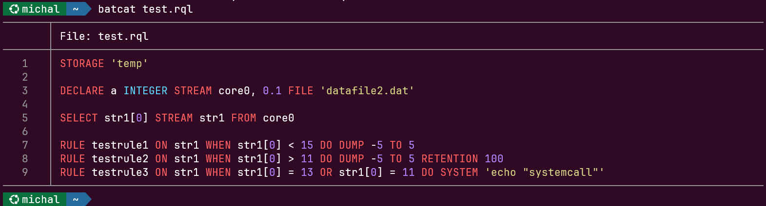
Fig. 66. RQL syntax highlighting in the terminal - the batcat command
Integration Tests
Integration tests verify the system’s behavior as a whole - they run the actual binaries (xretractor, xqry, xtrdb) and compare their output against patterns, or check specific properties of the output files. This differs from unit tests, which use the GTest framework to test isolated classes and functions of the rdb and retractor libraries (e.g. payload, descriptor, crsMath, compiler), don’t require a running server, and don’t produce artifacts on disk. Integration tests are run with the command ninja test (or ctest) in the build/Debug/ directory; a single test can be run with ctest -R <name> -V.
All scenarios live in one test/IntegrationTest directory. CMake assigns most directories one of sixteen RDB_NAMESPACE namespaces and its corresponding resource lock. This separates the bus, instance name, IPC objects, and log file without changing queries or patterns. Tests within one directory remain mutually exclusive, but different directories can run servers concurrently. Scenarios examining the production global identity, cooperation between several servers, or leftover cleanup (leftover_sweep) retain RUN_SERIAL: a concurrent instance could otherwise remove the leftovers before the assertions examine them.
The tables below describe the intent of each scenario. They are not an executable inventory: one directory usually registers several ctest entries (-run, -compile, -vg, and named variants), and the list grows with every release. The current state is returned by ctest -N in the build/Debug directory.
After the directory merge, all integration tests use the it_ prefix; the former pt_ prefix no longer denotes a separate class. Script tests use st_, while API tests also carry the api label and are skipped by ninja test by default. Two top-level guards - harness_guard-selftest and harness_command_integrity - verify that a wrapper actually ran the command under test and did not mask its exit status.
Valgrind descriptions refer to the standard Linux run. The Apple development port runs tests without that wrapper and requires a separate sanitizer build; a -vg name does not establish memory checking. See Apple development environment for the test scope and explicit test-api step. Unit tests in test_busFallback.cpp also check that a stopped live owner retains its lock and that the lock is recovered after its owner dies.
Execution and service scenarios
| Test name | Description |
|---|---|
Data | A shared set of data and queries for cross-cutting scenarios: waterfall (a full plan run under -m 10 plus artifact cleanup), workflow (a reference query, comparing two result streams), and all-operators (the same run for a query using the complete set of algebra operators). See: Data Processing and Distribution. |
ipc_identity_lock | A held IPC identity rejects startup before storage is changed; two servers with the same explicit name cannot take over shared IPC despite different TMPDIR values and bus namespaces. The first server remains responsive. It takes the lock through the engine’s own protocol (stillLinked with retries), because a bare open() plus flock() lost the race against a neighbouring test’s sweeper. Every failed check dumps the state at the moment of failure - the contents of /dev/shm with inodes, the locks with their owners from /proc/locks, the process table, and the tail of the engine log - which is why the test runs in parallel, without RUN_SERIAL. |
leftover_sweep | Cleanup after normal exit, restart following SIGKILL, exit of another instance, and explicit --cleanup. Checks that a live server retains its resources. Runs serially so a concurrent process cannot remove the leftovers under examination. |
agse1 | The @(start, length) time-window operator - forward variants @(1,4), backward @(1,-4), various lengths. See: AGSE Sliding Data Window. |
agse_array | AGSE over a numeric array field and an equivalent scalar schema: every flat element must enter the window in the same order. See: Aggregate Operators, Compilation Passes. |
agse_volatile | An AGSE window over a VOLATILE stream (MEMORY buffer) must see the whole window range. With too small a capacity the ring buffer overwrites the oldest field and the window reads the newest record in its place. See: VOLATILE Clause, AGSE Sliding Data Window. |
array_derived | Equivalence between numeric T[N] and explicit scalar fields through copy, shift, AGSE, SUMC, interleave, and mixed interleave, including NULL mapping. See: Aggregate Operators, Compilation Passes. |
client_tty_keystroke_immunity | A byte waiting on a pseudoterminal must not shorten xqry --elimitqry N reception; the client must receive its complete record budget before executing the combined --kill. |
config_storage_validation | Hard rejection of an invalid storage.dir in the TOML file: the nonexistent variant (directory missing) and unwritable (no write permission). In both the program exits non-zero with a Configuration error: storage.dir … message. The config-errors variant checks a discovered layer with invalid TOML syntax and with a relative paths.lock_dir in xretractor, xqry and xtrdb (nonzero exit code, file name and cause on stderr), a missing file as the positive control, an explicit --config, and --help working despite a malformed configuration. See: Command-Line Options - xretractor, Configuration file. |
deinterleave_roundtrip | Bit-exact verification of the interleave–deinterleave round-trip identity: a2 and b2 recover the components exactly, from record zero, with no placeholder record. The patterns are derived from the formal definitions, not from engine output. See: Tails, Logical Origins and Operator Observability. |
device_timeout | Reading a DEVICE source without blocking, with a FIFO as a controlled source: an explicit TIMEOUT clause in the -c listing, a warning about a deadline longer than the rate, refusal of TIMEOUT on the deprecated FILE and of a negative [sources] timeout_s; deadline precedence (RQL, configuration, 0, -f mode); the same bytes as BINFILE and as DEVICE give the same results behind multi-rate operators; a FIFO without a writer starts without hanging and gives NULL records; --until-eof ends when the writer leaves, with no NULL record from beyond the end; xqry answers while the engine waits for the source; TIMEOUT survives an ad hoc import and --reset. -vg- variant under Valgrind. See: DECLARE Command. |
ecg_qrs | Full execution of the compact ECG pipeline: windows directly in FROM, [_] expansion based on their width, and function-form reducers. The test checks origin= and tail= in the plan and 4,830 records of deterministic content across four intermediate and final streams. See: MIT-BIH ECG Visualization, Underscore Symbol Processing, Tails, Logical Origins and Operator Observability. |
agse2 | Window @(n,m) combinations on a 3-field stream, alignment and rate conversion at ratios 1:1, 1:2, 2:3, 2:4. See: AGSE Sliding Data Window. |
agse3 | The @(n,m) operator when the output rate is lower than the input rate (source rate 0.1) - windows @(3,2), @(3,3), @(3,-3). See: AGSE Sliding Data Window. |
consistency | Read consistency: two streams read the same source; their difference must always equal 100. See: Data and Control Flow. |
fatal_exit_path | A fatal startup or communication-thread error exits with status 1, removes IPC and the service lock, and does not turn into SIGSEGV or SIGABRT. See: Data and Control Flow. |
fncall_runtime_case | Executes mathematical functions in forms accepted by the grammar, including Sqrt, Ceil, and Floor; the test verifies runtime values, not only successful compilation. See: Field Expressions and Scalar Functions. |
index_wildcard_mixed | Expansion of [_] as one mixed SELECT-list item: field order before and after the expansion, two independent expansions, and payload layout matching the hand-written reference. |
adhoc_parse_error | Invalid syntax, multiple statements, an out-of-range literal, a zero interval, and other invalid values are rejected with a reason without stopping the server or changing its plan. |
adhoc_rule | Attaching RULE ... DO DUMP at run time, the available-history boundary, and rejection of DO SYSTEM and a range deeper than the MEMORY store. |
issue202_hash_shift_e2e | Runtime verification of (A>2)#(B>1) = (A#B)>3 for ΔA=0.1 and ΔB=0.2: independent text sources, physical equality of the matched and CC streams, and comparison with the sequence derived from the interleave formula. See: Substrates. |
issue113_meta_internal | Structure of the .meta sidecar file: header size (8 B), entry size (18 B), sampling interval, null bitsets for records with and without nulls. See: Data Storage Format - Files. |
issue113_meta_xtrdb | Verification via xtrdb that after running xretractor+xqry, the .meta file is created and reported correctly (meta: temp/str_null.meta). See: Data Storage Format - Artifact Analysis. |
issue113_null_skip | The -n flag in xqry - rows that are entirely null are skipped; without the flag, all rows (including all-null ones) must be present. See: Command-Line Options - xqry. |
issue113_null_xqry | Nulls transmitted over IPC: null values from the source file are shown as null in xqry output. See: Command-Line Options - xqry. |
issue121_isnull | The isnull(field) function - returns 1 when the field is null, 0 otherwise. See: Field Expressions and Scalar Functions. |
issue121_null_propagation | Propagation of null values through SELECT to the output stream. See: SELECT Command. |
issue128_numeric_to_string | Conversion of INTEGER/FLOAT to STRING via the to_string() function with a declared field width; verification of the output descriptor. See: Field Expressions and Scalar Functions. |
issue128_string_to_numeric | Conversion of STRING to numeric types: to_integer(), to_float(), to_double(); null propagation through the conversion. See: Field Expressions and Scalar Functions. |
issue167_dedup_cascaded | Cascaded absorption of substrates via deduplicateSubstrats() - multi-step rewriting of PUSH_ID tokens. See: Substrates. |
issue167_dedup_field_names | Substrate deduplication without comparing schema field names - merging when field types are equivalent, regardless of names. See: Substrates. |
issue167_dedup_nonzero_offset | Updating PUSH_ID in the consumer’s lSchema for a non-zero offset of the absorbed substrate; coverage of the code path in compiler.cpp. See: Substrates. |
issue167_dedup_positive | The basic deduplication case: a substrate merged with a named stream with an equivalent program and field types. See: Substrates. |
issue167_triarg | Multi-argument stream expressions: s1+s2+s3, (s1#s2)#s3, s1+(s2#s3), s1+s2+s3+s4; in-memory and on-disk substrates. See: Substrates, Operation Sequencing. |
issue217_client_diag_stderr | xqry diagnostics must go to stderr, not stdout. Invoking it with no server running exits non-zero and leaves stderr non-empty - without that, redirecting >/dev/null 2>err made every client failure invisible. See: Command-Line Options - xqry. |
issue227_join_alignment | Separation of the logical origin from the tail. The run variant checks the origin= and tail= values printed by the compiler and the content of a window joined with its own source; the adhoc-origin variant checks that a query attached at run time starts at the slot in which the runtime saw it. Expected values are derived from the operator definitions. See: Tails, Logical Origins and Operator Observability, Ad Hoc Queries. |
issue42_rule | The RULE command - conditional DUMP and SYSTEM actions triggered on stream values; runs xretractor and reads the result via xtrdb. A separate -dump entry decomposes the temp/str1_*_dump*.tmp files into INTEGER values and compares them against a pattern - it pins the actual state, including the leading zeros that DO DUMP -5 writes over a stream younger than six records. See: RULE Command. |
k19_boundaries | Operator observability boundaries: forward and backward windows, difference at equal and doubled interval, .sumc reduction. Distinguishes a genuine NULL inside a full window from the internal all-null record returned as a failsafe when reading outside the retained history. See: Tails, Logical Origins and Operator Observability. |
k24_capacity | History depth for operators that read ahead. Differences at an integral ratio ≥ 3 previously produced a stream of correct length consisting entirely of all-NULL records (a silent defect), and a chain of window, shift, and interleave ended in process abort inside storage::revRead. See: Compilation Passes. |
k24h10_exact_tails | Emission boundaries for difference and both de-interleaves, including sources with non-zero tails. Record count and content guard the exact phase rules against premature or delayed emission. See: Tails, Logical Origins and Operator Observability. |
noclock_offline | Artifact and logical-timeline equivalence between paced and --no-clock execution, plus rejection of --no-clock --realtime. See: Command-Line Options - xretractor. |
multiserver_named | Two named instances, separate locks and IPC, every form of --name, automatic names, and independent shutdown. |
multiserver_no_clobber | A losing start of the same instance does not delete the owner’s artifacts and reports its PID. |
multiserver_routing | Automatic routing of streams, ad hoc commands, and RULE; rejection of cross-server requests; bus listing; and waiting for the correct instance. |
multiserver_uniqueness | Atomic uniqueness of stream names, storage files, and the rotation counter during startup, ad hoc attachment, service delivery, and concurrent starts. |
null_divide_by_zero | Division by zero is an absorbing value: the stream yields NULL and keeps running. The point of the test is the record following the division - had the missing result been handled by an exception, it would never have been produced. See: Field Expressions and Scalar Functions. |
issue56_timeshift | The > filter operator on joined streams - only records satisfying the condition end up in the output stream. See: SELECT Command - Sequencing. |
issue61_tmpmem | The in-memory substrate SUBSTRAT 'memory' - intermediate data kept in RAM instead of on disk. See: STORAGE Types. |
issue6_adhoc | Ad-hoc query mode: xqry -a 'SELECT ...' - defining and executing a query on the fly, without an .rql file. See: Ad Hoc Queries. |
operations | The # (HASH merge) operator on two streams with different rates - verifying the ratio of record counts in the output. See: Interleaving Operation Sequencing. |
optimizer_ablation | Variant builds with individual optimizer rules switched off. build-info checks the identity of the configuration the binary reports, plan checks plan shape, and the remaining variants (semantic, factor-*, dedup-*) compare execution results across configurations. Every admissible optimizer configuration must preserve the observable result. See: Production Builds and Diagnostic Variants. |
packaging | Checks the exact DEB contents when dpkg-deb is available: three binaries, systemd unit, license, default TOML, and configuration examples. Separately checks portable TGZ: three binaries, license, and default TOML, with relative paths and no service. Source packages are disabled and are not tested. See: Production Builds and Diagnostic Variants. |
r1_identity_nulls | The R1 identity for the rewritten plan, blocked/non-rewritten left-hand side, and explicit right-hand side: equal origin=, payload, and NULL map in .meta. The non-rewritten side has a strictly larger tail - R1 preserves the record sequence, not the latency - so its comparison covers the common prefix. The ΔA/ΔB=3/2 case guards the phase-maximum own tail of #. See: Substrates. |
replay_stability | Repeating the same plan on the same data must produce an identical set of non-empty artifacts: payloads, descriptors, NULL maps, and shadow files; only the 8-byte reserved header is omitted from metadata comparison. See: Stream Replay, Data Storage Format. |
rotation_test | The stream binary-file rotation mechanism (ROTATION) - file count after two xretractor -m 2 cycles. See: File Rotation Mechanism. |
select_cse_commutative_add | Sharing equivalent SELECT computations for a+b and b+a: one STREAM_SELECT_*, separate public artifacts and descriptors, and identical data and NULL metadata. The test also guards SELECT *, projection order, and the three-source regrouping counterexample. See: Substrates. |
service_delivery | Delivering a set to a live service: correct target selection, startup-plan persistence, rejection on collision with another instance, and starting a separate instance when --name or --autoname is supplied. |
service_idle | Service and idle mode: starting without an .rql file completes cleanly, and the log goes to stderr in sd-daemon format (priority prefix, no timestamp). Two ways of enabling it - the --service flag and the XRETRACTOR_SERVICE variable. See: General Perspective, Command-Line Options - xretractor. |
service_reset | Two-phase replacement of a complete plan, preservation of the old plan after rejection, transitions to and from idle, and persistence of the service startup plan. It also covers the DO SYSTEM boundary: a plan carrying such a rule is refused as a whole, the refusal names the rule and the reason, the rule does not run, and the old plan keeps computing - and the same plan is accepted, with the rule working, once the unrestricted.toml configuration sets service.unrestricted = true. |
service_reset_double | Two consecutive plan replacements on the same instance and correct reconstruction of resources for the next epoch. |
service_reset_race | Concurrent reset and client commands never observe a partially dismantled or partially active plan. |
show_handler_failure | A failure in the server’s show subscription handler reaches the client as the direct rejection reason instead of appearing later as a response-queue timeout. |
simple | A smoke test for arithmetic on joined streams (core0 rate 0.1 + core1 rate 0.2), read via xtrdb. See: SELECT Command. |
simple_max | The backward-compatible, deprecated .max notation - the maximum value, joined with the original stream. See: Aggregate Operators. |
slot_schedule | Slot schedule against a fixed anchor, measured by the moments at which records appear in the store: slot work shorter than the period (waiting for an empty DEVICE and a DO SYSTEM rule) does not make the delay grow, also with --realtime; after a single stall the overdue slots run without sleeping, execution returns to the original grid, and the BINFILE and DEVICE artifacts are byte-identical to a --no-clock run; a new epoch after --reset has its own anchor; an ad hoc import of a new rate does not shift the axis; SIGTERM during the sleep ends the run immediately, without a slot before its deadline. A -vg- variant runs under Valgrind (drift and catch-up, period 1/4 s). See: Query Tree Traversal Algorithm. |
source_kinds | Source kind from the keyword, not from the path: BINFILE 'ascii.txt' reads raw bytes, TEXTFILE 'values.dat' parses text with the NULL token, DEVICE on a FIFO named .txt reads raw bytes, and a zero byte is not NULL. File kind refusals (FIFO without a writer, character device, regular file for DEVICE) with exit code 71 and without hanging. Without --verbose the deprecated FILE form gives output identical to the explicit keywords, with --verbose one warning per declaration - also on an ad hoc import. Source descriptor: the old TYPE DEVICE of a binary file is replaced, a change of kind or path is refused. A -vg- variant runs under Valgrind. See: DECLARE Command. |
stream_generator | The SELECT ... STREAM cell[N] generator: executing the family matches manually written-out streams, the instances are named cell$0…cell$(N-1), and cleanup removes the artifacts of the whole family. See: SELECT Command - Stream Generators. |
string_field_passthrough | Unquoted TEXTSOURCE input, neighboring-field alignment, STRING[N] clipping, type propagation, and the actual value measured by Length. See: Field Expressions and Scalar Functions, Compilation Passes. |
tty_keystroke_immunity | A byte waiting on a pseudoterminal must not shorten xretractor --llimitqry N; a run under a TTY must produce the same amount of data as a run without a terminal. |
untileof_stop | --until-eof matches a manually bounded ONESHOT source, does not wrap the file, and stops at the first exhausted source in a multi-source plan. See: Command-Line Options - xretractor. |
wide_from_names | A wide FROM clause past the 200-byte threshold uses a stable shortened substrate name, stays within NAME_MAX, preserves deduplication, and performs the SUMC reduction over the window correctly. See: Substrates. |
window_aggregate | Record-history MIN/MAX/AVG/SUMC(expression : W): values, types, boundaries, arrays, expressions, shared groups, NULL, null2zero, and schema propagation through a copy. See: Aggregate Operators. |
xqry_array_row | Complete serialization of a numeric array field by xqry: every element in order in raw, Graphite, and InfluxDB formats, without limiting the value count to the number of descriptor entries. See: Command-Line Options - xqry, Stream Monitoring API. |
xqry_elem_limit | The -m N parameter in xqry - limits the number of received records to exactly N, regardless of the source’s length. See: Command-Line Options - xqry. |
xqrywait_gate | The --xqrywait gate does not lose the first command, does not reset the --llimitqry budget, and can be interrupted by a signal before a client arrives. |
Newer regression scenarios
| Test name | Description |
|---|---|
adhoc_register_rollback | A forced ad hoc registration failure restores the plan and bus claims; the server keeps processing and the retried query works. |
expr_corpus | Eleven expression plans, including mixed types and strings, check values and types against patterns and an independent oracle. |
ipc_client_killed_reading | Killing a client while it reads a response does not block later commands. |
issue252_missing_stream | A request for an unknown stream returns a refusal while the server keeps emitting records. |
rule_string_compare | String comparisons and a bare string condition in RULE WHEN fire rules in the correct slots. |
xtrdb_engine_guard | xtrdb refuses access for a live named instance, including one using a custom paths.lock_dir, but accepts a stale lock file. |
expr_result_types | Result-field types and sizes, fractional values, NULL, and schema copying through SELECT *. |
field_ref_outside_from | Rejects a reference to a field of a stream outside FROM and verifies a reference through the result stream’s field. |
reducer_field_ref | Rejects a reducer name used as a field in SELECT and reads the result through a materialized stream. |
reducer_float_max_avg_count | MAX over negative FLOAT and DOUBLE values, and AVG over records with 256 and 257 fields. |
self_ref_field_shape | A field referenced by the stream’s own name takes its type from the corresponding FROM record slot. |
self_ref_simplify_synth | Input-slot types for windows and reducers protect FLOAT calculations from incorrect constant simplification. |
self_ref_simplify_type | A self-reference in an expression eligible for simplification uses the FROM slot type, not the output-field type. |
silent_arith_overflow | Overflow in INTEGER and RATIONAL expressions and reducers yields NULL instead of a wrapped number. |
synth_node_output_shape | Output-field types after a window, reducer, or join match the actual input slots. |
xqrywait_first_row | The first record survives the interval between opening the --xqrywait gate and creating the xqry subscription queue. |
Compilation and offline scenarios
The following directories primarily register compilation variants, plan presentation, or artifact operations. Some also occur in the execution table because one CMakeLists.txt can register several independent CTest entries.
| Test name | Description |
|---|---|
Data | The compilation side of the shared Data set (files shared with the serial variant): on-query - compilation of the reference query, presenter - plan presentation after that compilation, banned-artifacts - a guard checking that no artifact with a forbidden name colliding with system tools was created in the install directory. See: Compilation and Plan Construction. |
dsp | Compilation regression for the compact FIR filter pipeline: the source@(1,25) window directly in FROM, 25-element expansion of source[_] * filter[_], the SUMC(accRow) reduction, and joining the signal with the output. See: Signal Filter Implementation, Underscore Symbol Processing. |
issue113_meta | xtrdb operations after two appends - record list and hexdump of the binary file compared against a pattern. See: Data Storage Format - Artifact Analysis. |
issue113_meta_autocreate | Automatic creation of the .meta sidecar file after the first append; size >16 B; xtrdb reports the correct path. See: Data Storage Format - Files. |
issue113_null_txtsrc | The rread/getpos commands in xtrdb on a TEXTSOURCE stream containing nulls. See: Data Storage Format - Artifact Analysis. |
issue153_storagemap_meta_cases | The xtrdb -s storage map for a plain file and a retractordb-style file: slot markers, segment list, rotated files, .meta/.shadow references. See: Inspection Tool xtrdb -s. |
issue202_hash_shift_factorization | Algebraic optimization of (A>i)#(B>k) into (A#B)>(i+k) when i·ΔA=k·ΔB, plus protection of the unmatched case. See: Substrates. |
issue31_doc | Generating DOT/SVG graphs via xretractor -c -d ... for documentation examples at three levels of detail. See: Compilation Debugging. |
issue42_rule | Compilation of RULE syntax - the -c stage only, without starting the server. See: RULE Command. |
issue56_timeshift | Compilation of the > filter operator - the -c stage only. See: SELECT Command - Sequencing. |
issue61_tmpmem | Compilation of a query with SUBSTRAT 'memory' - the -c stage only. See: STORAGE Types. |
issue95_loopInCompile | Cycle detection in the query graph by the compiler - expected “Circular dependency” error and a non-zero exit code. See: Loop Detection in Compilation. |
issue96_no_substrat_reduction | User-defined streams with an identical structure are NOT merged; only automatic substrates are subject to merging. See: Substrates. |
issue96_substrat_reference | A generated substrate shared by two user streams - correct references in the dependency tree. See: Substrates. |
Pattern1 | Compilation of the # (HASH-merge) operator, field selection with an offset, and stream joining with +. See: Interleaving and Summation Operation Sequencing. |
Pattern2 | Compilation of queries on BYTE streams from /dev/urandom: SELECT, arithmetic, stream joining. See: SELECT Command. |
Pattern3 | Compilation of SELECT * (unfold) with an output-file declaration and retention. See: Asterisk Expansion. |
Pattern5 | xtrdb operations on a multi-type record (STRING, INTEGER, BYTE, FLOAT): append, read, list/rlist, input, write. See: Artifact Analysis. |
Pattern6 | Compilation of the window operator @(n,m) forward @(1,10) and backward @(1,-10), plus a leak-free valgrind run. See: AGSE Sliding Data Window. |
Pattern7 | Compilation with identical field names across multiple streams (issue #17) - correct field identification via the stream index. See: DECLARE Command, Aliasing. |
retention | xtrdb operations on a file with a RETENTION parameter: open, purge, append, list, write for a specific record. See: Data Storage Format - File Rotation Mechanism. |
simple | Compilation of a basic arithmetic query + DOT graph + valgrind; uses data from IntegrationTest/simple. See: SELECT Command. |
simple_max | Compilation of a query with .max + DOT graph + valgrind; uses data from IntegrationTest/simple_max. See: Aggregate Operators. |
subquery | Compilation of nested subqueries: (a#b)>1 (hash-merge inside a filter) and (a>1)#b (filter inside a hash-merge). See: Dependency Tree Construction. |
txtsrc | xtrdb operations descc/rread/printt on a TEXTSOURCE stream (a text file as a data source). See: Data Storage Format. |
Installation Process
RetractorDB’s primary deployment platform is Linux on x86-64 and ARM64 (AArch64). You can install a release package or build the programs from source. The installer downloaded with curl installs prebuilt binaries; compilation is a separate operation. Apple is a development environment, covered in a separate section.
Choosing an installation method
| Method | Use | Binary location |
|---|---|---|
Installer install.sh --user | Installation for the current user, without administrator privileges | ~/.local/bin |
Installer install.sh --system | System-wide installation, optionally with a systemd service | /usr/local/bin |
| DEB package | Debian or Ubuntu; managed through apt | /usr/bin |
| Building from source | Development, testing, or your own release | ~/.local/bin by default |
The installer uses GitHub Releases. A quick installation guide is also available on the project website. The production-build contract and diagnostic variants are described in the build appendix.
Installing a release on Linux
The installer requires Bash, curl, python3, and sha256sum. It detects x86-64 and AArch64, selects a retractordb-<version>-linux-<architecture>-portable.tar.gz archive, and verifies its SHA-256 against the GitHub release asset’s digest field. Before installation it checks the archive contents, ELF architecture, and whether all three programs can run. A system with an incompatible glibc or libstdc++, a musl-based distribution, or 32-bit ARM may require a separate source build.
To check the releases available for the host architecture:
curl -fsSL https://retractordb.com/install.sh | bash -s -- list
By default, the newest stable version with a matching archive is selected. Drafts and prereleases are skipped. To install for the current user:
curl -fsSL https://retractordb.com/install.sh | bash -s -- install --user
The xretractor, xqry, and xtrdb programs are available through links in ~/.local/bin. If that directory is missing from PATH, add it to your shell configuration. The installer prints this advice but does not change the shell configuration itself.
You can also download and inspect the script first:
curl -fsSLO https://retractordb.com/install.sh
less install.sh
bash install.sh install --user
System installation and the systemd service
System installation requires root privileges and uses the /usr/local prefix:
curl -fsSL https://retractordb.com/install.sh | sudo bash -s -- install --system
On a host running systemd, --service also installs, enables, and starts the service:
curl -fsSL https://retractordb.com/install.sh | sudo bash -s -- install --system --service
systemctl status xretractor.service
The installer creates the retractor account and an empty /etc/retractor/startup.rql if they do not already exist. An empty file starts an idle instance ready to accept a plan. Existing queries are preserved. The service prefix must be owned by root and must not be writable by other users. The portable archive itself contains no systemd unit; the installer creates it.
Ways to deliver a plan to a running service are described in the xretractor options.
Upgrades, versions, status and removal
curl -fsSL https://retractordb.com/install.sh | bash -s -- upgrade --user
curl -fsSL https://retractordb.com/install.sh | bash -s -- status --user
curl -fsSL https://retractordb.com/install.sh | bash -s -- uninstall --user
install and upgrade accept --version <version> with a release number available through list. Use --prefix /absolute/path for a custom directory; supply the same prefix when upgrading, checking, or removing it. For a system installation, use --system and run operations that modify the installation as root.
The installer stores programs in <prefix>/lib/retractordb/versions/<version> and maintains an installer-state file in <prefix>/lib/retractordb. The status command shows the managed installation and binary links; it does not check whether the engine is ready to handle queries. Use a command such as xqry --server service --hello to contact a running instance.
An upgrade restarts the managed systemd service with the new binary. uninstall removes the programs and its own unit while preserving configuration, query files, and the service account. The installer does not take over binaries installed by another method in the same prefix; choose a separate prefix or keep using the original installation method.
Stop running instances before updating their binaries. Versions using different bus layouts have separate registries and do not provide shared collision checks for stream names or storage paths. The current layout is described in Multiple Instances and the Bus.
DEB package
For Debian or Ubuntu, download a DEB package matching the architecture from GitHub Releases and install it through apt. In the example below, package.deb denotes the downloaded file:
sudo apt install ./package.deb
The package installs programs in /usr/bin, prepares configuration, and enables the service for the next system boot. To start it immediately:
sudo systemctl start xretractor.service
systemctl status xretractor.service
Upgrade with apt install ./<new-file>.deb and remove with sudo apt remove retractordb. The portable installer does not manage Debian packages. Do not install both the DEB variant and the portable variant with --service on one host: both use the xretractor.service name.
Building and installing from source
Linux builds use Conan 2, CMake, and Ninja. A C++23 compiler with <print> and std::println is required (GCC 14 or newer). The project’s toolchain requires CMake 4.4.2 or newer. The scripts/buildrdb.sh script prepares the tools and Conan profile; dependency installation on Linux uses apt.
From the downloaded retractordb repository:
scripts/buildrdb.sh toolchain
scripts/buildrdb.sh conan ninja
scripts/buildrdb.sh bashrc
After adding ~/.local/bin to PATH, refresh the shell, for example by opening a new terminal. To build and install Debug:
scripts/buildrdb.sh debug
cmake --install build/Debug
ctest --test-dir build/Debug --output-on-failure
Installation is a separate step after building and does not require sudo by default. Integration tests also use installed programs, so installation precedes testing. The optional API libraries have separate installation and test targets.
A production release from source requires a clean Git tree:
scripts/buildrdb.sh release
cmake --install build/Release
ctest --test-dir build/Release --output-on-failure
The release-dirty mode is for diagnosing local changes and does not produce a production release. See the build contract. Packages for distribution are prepared separately; scripts and checks for Linux releases are described in the code repository’s scripts/release_package/README.md.
Checking the installation and configuration
xretractor --build-info
xqry -h
xtrdb -h
--build-info shows the binary’s optimizer flags without starting the engine. It does not replace testing your own plan. After installation, also check command -v xretractor to confirm that PATH selects the intended installation.
The portable installer copies the default TOML only if the file is absent: to /etc/retractor/retractor.toml for a system installation or $XDG_CONFIG_HOME/retractor/retractor.toml (by default ~/.config/retractor/retractor.toml) for the user. The shipped file leaves storage.dir commented out. Before setting it, create the directory and grant write access to the user running the engine. The complete configuration order and RQL directive precedence are described in the xretractor options.
Installation through cmake --install places the default TOML in <prefix>/share/retractordb/retractor.toml; it does not activate it as user configuration. You can copy it to your configuration location or select it with --config.
An operator can bound RAM history and growth of DEFAULT/DIRECT file streams without their own retention:
[limits]
history_memory_mib = 1024
[storage]
default_retention = [1000, 4]
history_memory_mib is a positive MiB budget for sources and MEMORY rings; a larger plan is rejected at compilation. default_retention requires two positive numbers [capacity, segments], also applies to file-based substrates, and does not override explicit RETENTION. Without it, file streams without retention still grow; xretractor lists them at startup and in -c. The TOML file may also contain server.autoname (default false) and service.unrestricted (default false, allowing DO SYSTEM through xqry --reset); their effects and precedence are explained in the xretractor options.
Apple development environment
The macOS port is for development and testing. The system’s general contract, service description, and production procedures in this manual apply to Linux. The curl installer described above supports Linux; Apple requires a source build.
The tested port configuration is Apple silicon with macOS 27 and Apple clang 21. Intel Macs and older system releases remain unverified. Xcode 16.3+ Command Line Tools and a macOS 14.4+ deployment target are minimum requirements imposed by std::print, not a declaration that all such configurations have been tested.
Before building, prepare the Command Line Tools (xcode-select --install), Homebrew, and CMake, Python 3, and Git available on PATH. On macOS, scripts/buildrdb.sh toolchain uses Homebrew. The script below can install missing Conan and Ninja through Homebrew; it also uses the Conan environment to provide the required CMake version:
scripts/macos-build.sh
scripts/macos-build.sh --sanitize
The default run is Debug: configure, build, install, refresh the test copy, rebuild, run CTest, and run the separate test-api target. The log is written to build/macos-build.log. --sanitize enables AddressSanitizer and UndefinedBehaviorSanitizer. --no-install disables automatic tool installation, but still installs the built programs. --skip-tests skips tests while retaining installation. scripts/macos-build.sh release selects the Release configuration but does not perform the checks of the production scripts/buildrdb.sh release workflow.
Differences relevant to development
| Area | macOS port behavior |
|---|---|
| Configuration | Without --config, layers are read in order from /etc/retractor/retractor.toml, /usr/local/etc/retractor/retractor.toml, /opt/homebrew/etc/retractor/retractor.toml, then the user location. Later layers override earlier keys. The Homebrew path does not imply that an installation formula is available. |
| IPC | Boost.Interprocess uses file-backed storage under /tmp/boost_interprocess/...; --shmbudget reports that volume rather than Linux’s /dev/shm tmpfs. Overlong object names receive a deterministic shortened token; the public server name retains its 32-character limit. |
| Process liveness | sysctl provides the PID and start time; the absence of /proc does not remove the live-owner check. The bus lock has a fallback that recovers after its owner’s death. |
| Real time | SCHED_FIFO is set on the processing thread through pthread_setschedparam. The TOML priority (1..99) is clamped to the kernel’s range. CPU affinity and a PREEMPT_RT equivalent are unavailable; mlockall can return ENOSYS, after which execution continues without locked memory pages. Absolute sleep uses the Mach interface. This is not a measurement platform for Linux real-time guarantees. |
| Service | The code identifies a launchd job through XPC_SERVICE_NAME and parent PID 1, and builds a restart command using launchctl kickstart -k. Choosing the domain from the effective UID is a heuristic: a system daemon running as a non-root user may receive the wrong domain. The package provides neither a .plist nor a launchd service installer. |
| Memory tests | On Apple silicon, tests run without Valgrind. Run memory checks in a separate sanitizer configuration; passing ordinary CTest, including entries with -vg in their names, does not establish that such checks ran. |
| API | The script explicitly runs test-api, covering Python and C++ clients and process creation. The API remains optional; this development path does not extend the production API contract to macOS. |
| Packaging | CPack creates TGZ without the systemd service component. The ability to create a Darwin archive locally does not mean it is available through the web installer. |
Platform capability checks and fallback declarations are described in the build appendix.
References
1. S. Beatty, “Problem 3173” American Mathematical Monthly, vol. 33, p. 159, 1926.
2. A.S.Fraenkel, “The bracket function and complementary sets of integers” Canadian Journal of Mathematics, vol. 21, pp. 6-27, 1969. (link)
3. M. Widera, “Deterministic method of data sequence processing” Annales UMCS, Sectio AI Informatica, vol. IV, pp. 314-331, 2006 (link); Polish version: “Deterministyczna metoda przetwarzania ciagow danych” in XXI Autumn Meeting of Polish Information Processing Society, Conference Proceedings, pp. 243-254, 2006. (pdf)
4. Z. W. Zen, “Classified publications on covering systems” updated 2006. [Online]. Available: http://maths.nju.edu.cn/~zwsun/. (pdf)
5. T. Parr, The Definitive ANTLR 4 Reference, The Pragmatic Bookshelf, 2013. (amazon)
6. T. D. Pauw, “Swirly - A marble diagram generator.” 2022. [Online]. Available: https://github.com/timdp/swirly. [Accessed: 3 Nov 2025]. (link)
7. A. Staltz, “RxJS Marbles” https://github.com/staltz/rxmarbles, [Online]. Available: https://rxmarbles.com/. [Accessed: 4 Nov 2025]. (link)
8. “Conan.io - the Open Source C and C++ Package Manager for Developers” JFrog, [Online]. Available: https://conan.io/. [Accessed: 9 Nov 2025].
9. D. W. Gunness, “Creating digital signal processing (DSP) filters to improve loudspeaker transient response”. US Patent US8081766B2, 20 Dec 2011. (link)
10. M. Widera, “RetractorDB - separator serii czasowych” Programista, vol. 92, no. 5/2020, pp. 14-20, 6/7 2020. (ebookpoint)
11. J. Shallit, “A Generating Function Technique for Beatty Sequences and Other Step Sequences” Journal of Number Theory, vol. 64, no. 2, pp. 273-298, 1997.
12. L. Schaeffer, J. Shallit and S. Zorcic, “Beatty Sequences for a Quadratic Irrational: Decidability and Applications” arXiv:2402.08331, 2024. (pdf)
13. M. A. Berger, A. Felzenbaum and A. S. Fraenkel, “Disjoint covering systems of rational Beatty sequences” Journal of Combinatorial Theory, Series A, vol. 42, no. 1, pp. 150-153, 1986.
14. D. Eppstein et al., “Aperiodic pinwheel scheduling using Beatty sequences” - a discussion of the periodic-scheduling problem based on complementary Beatty sequences, 2023. (link)
15. H. Fujiwara, K. Miyagi and K. Ouchi, “Pinwheel Scheduling with Real Periods” arXiv:2510.24068, 2025 - proofs based on the Rayleigh/Beatty partition, with identities on floor and ceiling functions. (html)
16. S. Samadi, M. O. Ahmad and M. N. S. Swamy, “Characterization of nonuniform perfect-reconstruction filterbanks using unit-step signal” IEEE Transactions on Signal Processing, vol. 52, no. 9, pp. 2490-2499, 2004. (link)
17. G. Margolis and Y. C. Eldar, “Nonuniform Sampling of Periodic Bandlimited Signals” IEEE Transactions on Signal Processing, vol. 56, no. 7, pp. 2728-2745, 2008. (pdf)
18. J. Kovačević and M. Vetterli, “Perfect Reconstruction Filter Banks with Rational Sampling Factors” IEEE Transactions on Signal Processing, vol. 41, no. 6, pp. 2047-2066, 1993.
19. S. Kalra and N. K. Shukla, “Ramanujan sums in signal recovery and uncertainty principle inequalities” arXiv:2512.16190, 2025. (pdf)
20. A. Arasu, S. Babu and J. Widom, “The CQL continuous query language: semantic foundations and query execution” The VLDB Journal, vol. 15, no. 2, pp. 121-142, 2006. (pdf)
21. J. Krämer and B. Seeger, “Semantics and implementation of continuous sliding window queries over data streams” ACM Transactions on Database Systems, vol. 34, no. 1, pp. 1-49, 2009 (the PIPES system).
22. S. K. Jensen, T. B. Pedersen and C. Thomsen, “Time Series Management Systems: A Survey” IEEE Transactions on Knowledge and Data Engineering, vol. 29, no. 11, pp. 2581-2600, 2017. (pdf)
23. K. O’Bryant, “Fraenkel’s partition and Brown’s decomposition” Integers: Electronic Journal of Combinatorial Number Theory, vol. 3, A11, 2003.
24. G. E. Pfander, S. Revay and D. Walnut, “Exponential bases for partitions of intervals” Applied and Computational Harmonic Analysis, vol. 68, art. 101607, 2024.
25. M. Widera, J. Jezewski, R. Winiarczyk, J. Wrobel, K. Horoba and A. Gacek, “Data stream processing in fetal monitoring system: I. Algebra and query language” Journal of Medical Informatics & Technologies, vol. 5, pp. 83-90, 2003.
26. E. A. Lee and D. G. Messerschmitt, “Static Scheduling of Synchronous Data Flow Programs for Digital Signal Processing” IEEE Transactions on Computers, vol. C-36, no. 1, pp. 24-35, 1987. (doi)
27. G. Bilsen, M. Engels, R. Lauwereins and J. A. Peperstraete, “Cyclo-Static Dataflow” IEEE Transactions on Signal Processing, vol. 44, no. 2, pp. 397-408, 1996.
28. A. Cohen, M. Duranton, C. Eisenbeis, C. Pagetti, F. Plateau and M. Pouzet, “N-Synchronous Kahn Networks: A Relaxed Model of Synchrony for Real-Time Systems” in Proceedings of the 33rd ACM SIGPLAN-SIGACT Symposium on Principles of Programming Languages (POPL), pp. 180-193, 2006. (doi)
29. F. McSherry, A. Lattuada, M. Schwarzkopf and T. Roscoe, “Shared Arrangements: Practical Inter-Query Sharing for Streaming Dataflows” Proceedings of the VLDB Endowment, vol. 13, no. 10, pp. 1793-1806, 2020. (doi)
30. A. Chaudhary, J. Karimov, S. Zeuch and V. Markl, “Incremental Stream Query Merging” in Proceedings of the 26th International Conference on Extending Database Technology (EDBT), pp. 604-617, 2023. (doi)